Simple Linear Regression
Multiple Linear Regression
Diagnostics in MLR: ANOVA, R^2, F-test
Potential issues with Linear Regression
Overview
Suppose we have pairs of data (y_1, x_1), (y_2, x_2), ..., (y_n, x_n) and we want to predict values of y_i based on x_i.
- We could do a linear prediction: y_i = {\color{magenta}{m}}x_i + {\color{blue}{b}}.
- We could do a quadratic prediction: y_i = ax_i^2 + bx_i + c.
- We could do any general functional prediction: y_i = f(x_i).
These are all examples of “models” we can specify. Let’s focus on the linear prediction. Some questions:
- How do we choose \color{magenta}{m} and \color{blue}{b}? Aren’t there infinite possibilities?
- How do we know whether our fitted line is a ‘good’ choice? What do we even mean by ‘good’?
Overview
In simple linear regression, we predict that a quantitive response “Y” is a linear function of a single predictor “X”, Y \approx \beta_0 + \beta_1 X.
“Simple” here refers to the fact there is a single predictor.
Assume we have n observations, and call \bm{y} = (y_1, ..., y_n)^\top the vector of responses and \bm{x} = (x_1,...,x_n)^{\top} the vector of correpsonding predictors. Our model states that the ‘true’ relationship between X and Y is linear (plus a “noise” or “error”). Using vector notation, we write: \bm{y} = \beta_0 + \beta_1 \bm{x} + \bm{\epsilon},
where \bm{\epsilon} = (\epsilon_1, ..., \epsilon_n)^{\top} is a vector of error terms (respecting certain assumptions).
Advertising Example
\texttt{sales} \approx \beta_0 + \beta_1 \times \texttt{TV}
![]()
Assumptions on the errors
Weak assumptions \mathbb{E}( \epsilon_i|\bm{x}) = 0,\quad \mathbb{V}( \epsilon_i|\bm{x}) = \sigma^2 \text{and}\quad Cov(\epsilon_i,\epsilon_j|\bm{x})=0 for i=1,2,3,...,n; for all i \neq j.
In other words, errors have zero mean, common variance and are conditionally uncorrelated. Those are the minimum assumptions for “Least Squares” estimation.
Strong assumptions \epsilon_i|\bm{x} \overset{\text{i.i.d.}}{\sim} \mathcal{N}(0,\sigma^2) for i=1,2,3,...,n. In other words, errors are i.i.d. Normal random variables with zero mean and constant variance. Those are the minimum assumptions for “Maximum Likelihood” estimation.
Model estimation
Recall we assume the ‘true’ relationship between X and Y (seen here as random variables) is described by Y =\beta_0 + \beta_1 X + \epsilon, where \epsilon satisfies either the weak or strong assumptions.
If we have an observed sample from (X,Y), say (x_1, y_1), ..., (x_n, y_n), we then want to obtain estimates \hat{\beta}_0 and \hat{\beta}_1 of the parameters \beta_0, \beta_1.
Once we have these estimates, we can predict any “response” simply by: \hat{y}_i=\hat{\beta}_0 + \hat{\beta}_1 x_i.
This makes sense because
\begin{aligned}
\mathbb{E}[Y|X=x_i] & = \mathbb{E}[\beta_0 + \beta_1 X + \epsilon_i | X=x_i] = {\beta}_0 + {\beta}_1 x_i
\end{aligned}
(where we used the fact that \mathbb{E}[\epsilon_i|X=x_i] = 0).
Least Squares Estimates (LSE)
- The most common approach to estimating \hat{\beta}_0 and \hat{\beta}_1.
- Minimise the residual sum of squares (RSS)
\mathrm{RSS} %= \sum_{i = 1}^{n} e_i^2
= \sum_{i = 1}^{n} (y_i - \hat{y}_i)^2 = \sum_{i = 1}^{n} (y_i - \hat{\beta}_0 - \hat{\beta}_1 x_i)^2
- The least square coefficient estimates are
\begin{aligned}
\hat{\beta}_1 &= \dfrac{\sum_{i = 1}^{n}(x_i - \bar{x}_i)(y_i - \bar{y}_i)}{\sum_{i=1}^{n}(x_i - \bar{x}_i)^2}=\frac{S_{xy}}{S_{xx}} \\
\hat{\beta}_0 &= \bar{y} - \hat{\beta}_1 \bar{x}
\end{aligned}
where \bar{y} \equiv \frac{1}{n}\sum_{i=1}^{n}y_i and \bar{x} \equiv \frac{1}{n}\sum_{i=1}^{n}x_i. See slide on S_{xy}, S_{xx} and sample (co-)variances. Proof: See Lab questions.
LS Demo
Least Squares Estimates (LSE) - Properties
- Under the weak assumptions we have unbiased estimators: \mathbb{E}\left[\hat{\beta }_{0}|\bm{x}\right] =\beta _{0} \quad \text{and} \quad \mathbb{E}\left[\hat{\beta }_{1}|\bm{x}\right] =\beta _{1}. Proof: See Lab questions.
- What does this mean? If the linear model is correct, the LSE are on average correct to estimate \beta_0 and \beta_1 (they don’t have a “systematic error”).
- Note an (unbiased) estimator of \sigma ^{2} is given by:
\begin{aligned}
s^{2} &= \frac{\sum_{i=1}^{n}\left( y_{i}-\left(\hat{\beta }_{0}+\hat{\beta }_{1}x_{i}\right) \right)^{2}}{n-2}.
\end{aligned}
- The next question is: how confident (or “certain”) are we in these estimates?
Least Squares Estimates (LSE) - Uncertainty
Under the weak assumptions we have that the (co-)variances of the parameters are:
\begin{aligned}
\text{Var}\left(\hat{\beta }_{0}|\bm{x}\right) =&\sigma^2\left(\frac{1}{n}+\frac{\overline{x}^2}{\sum_{i=1}^{n}(x_i-\overline{x})^2}\right)=\sigma^2\left(\frac{1}{n}+\frac{\overline{x}^2}{S_{xx}}\right)\\{ }=& SE(\hat{\beta_0})^2\\
\text{Var}\left( \hat{\beta }_{1}|\bm{x}\right) =& \frac{\sigma^2}{\sum_{i=1}^{n}(x_i-\overline{x})^2}=\frac{\sigma^2}{S_{xx}}=SE(\hat{\beta_1})^2\\ %= \frac{n\sigma^2}{nS_{xx}-S_{x}^2}\\
\text{Cov}\left( \hat{\beta }_{0},\hat{\beta }_{1}|\bm{x}\right) =& -\frac{ \overline{x} \sigma^2}{\sum_{i=1}^{n}(x_i-\overline{x})^2}=-\frac{ \overline{x} \sigma^2}{S_{xx}}
%%s_\epsilon^2 = \text{Var}\left(\hat{\epsilon}\right) =& \frac{nS_{yy}-S_y^2-\hat{\beta}_1^2(nS_{xx}-S_x^2)}{n(n-2)}
\end{aligned}
Proof: See Lab questions. Hopefully you can see that all three quantities go to 0 as n gets larger.
Maximum Likelihood Estimates (MLE)
- In a simple regression model, there are three parameters to estimate: \beta_0, \beta_1, and \sigma^{2}.
- Under the strong assumptions (i.i.d. Normal errors), the joint density of Y_{1},Y_{2},\ldots,Y_{n} (conditional on X_i=x_i, the values taken by the predictors) is the product of their marginals densities (because all the Y_i|x_i are independent, by assumption).
- So, the log-likelihood is:
\begin{aligned}
%L\left({y};\beta_0 ,\beta_1 ,\sigma \right) =&\prod_{i=1}^{n}\frac{1}{\sqrt{2\pi }\sigma }\exp \left( -\frac{\left(y_{i}-\left( \beta_0 +\beta_1 x_{i}\right) \right) ^{2}}{2\sigma ^{2}}\right)\\
%=&\frac{1}{\left( 2\pi \right) ^{n/2}\sigma ^{n}}\exp \left( -\frac{1}{2\sigma ^{2}}\sum_{i=1}^{n}\left( y_{i}-\left( \beta_0 +\beta_1 x_{i}\right) \right) ^{2}\right)\\
\ell\left({y};\beta_0 ,\beta_1 ,\sigma \right) =&-n\ln\left( \sqrt{2\pi} \sigma\right) -\frac{1}{2\sigma^{2}}\sum_{i=1}^{n}\left( y_{i}-\left( \beta_0 +\beta_1 x_{i}\right) \right) ^{2}.
\end{aligned}
Proof: Since Y_i|x_i = \beta_0 + \beta_1 x_i + \epsilon_i, where \epsilon_i \overset{\text{i.i.d.}}{\sim} \mathcal{N}(0,\sigma^2), then Y_i|x_i \overset{\text{i.i.d.}}{\sim} \mathcal{N}\left( \beta_0 + \beta_1 x_i, \sigma^2 \right). The result follows.
Maximum Likelihood Estimates (MLE)
Partial derivatives set to zero give the following MLEs:
\begin{aligned}
\hat{\beta}_1=&\frac{\sum_{i=1}^{n}\left( x_{i}-\overline{x}\right)
\left( y_{i}-\overline{y}\right) }{\sum_{i=1}^{n}\left( x_{i}-\overline{x}\right) ^{2}}=\frac{S_{xy}}{S_{xx}},\\
\hat{\beta}_0=&\overline{y}-\hat{\beta}_1\overline{x},
\end{aligned}
and
\hat{\sigma }_{\text{MLE}}^{2}=\frac{1}{n}\sum_{i=1}^{n}\left( y_{i}-\left( \hat{\beta}_0+\hat{\beta}_1x_{i}\right) \right) ^{2}.
- Note that the parameters \beta_0 and \beta_1 have the same estimators as that produced from Least Squares.
- However, the MLE \hat{\sigma}^{2} is a slightly biased estimator of \sigma^{2}.
- In practice, we use the unbiased version s^2 (see slide).
Interpretating the parameters
How do we interpret a linear regression model such as \hat{\beta}_0 = 1 and \hat{\beta}_1 = -0.5?
- The intercept parameter \hat{\beta}_0 is interpreted as the value we would predict for y_i if x_i = 0.
- E.g., predict y_i = 1 if x_i=0
- The slope parameter \hat{\beta}_1 is the expected (or mean) change in the response y_i for a 1 unit increase in x_i.
- E.g., we would expect y_i to decrease on average of -0.5 for every 1 unit increase in x_i.
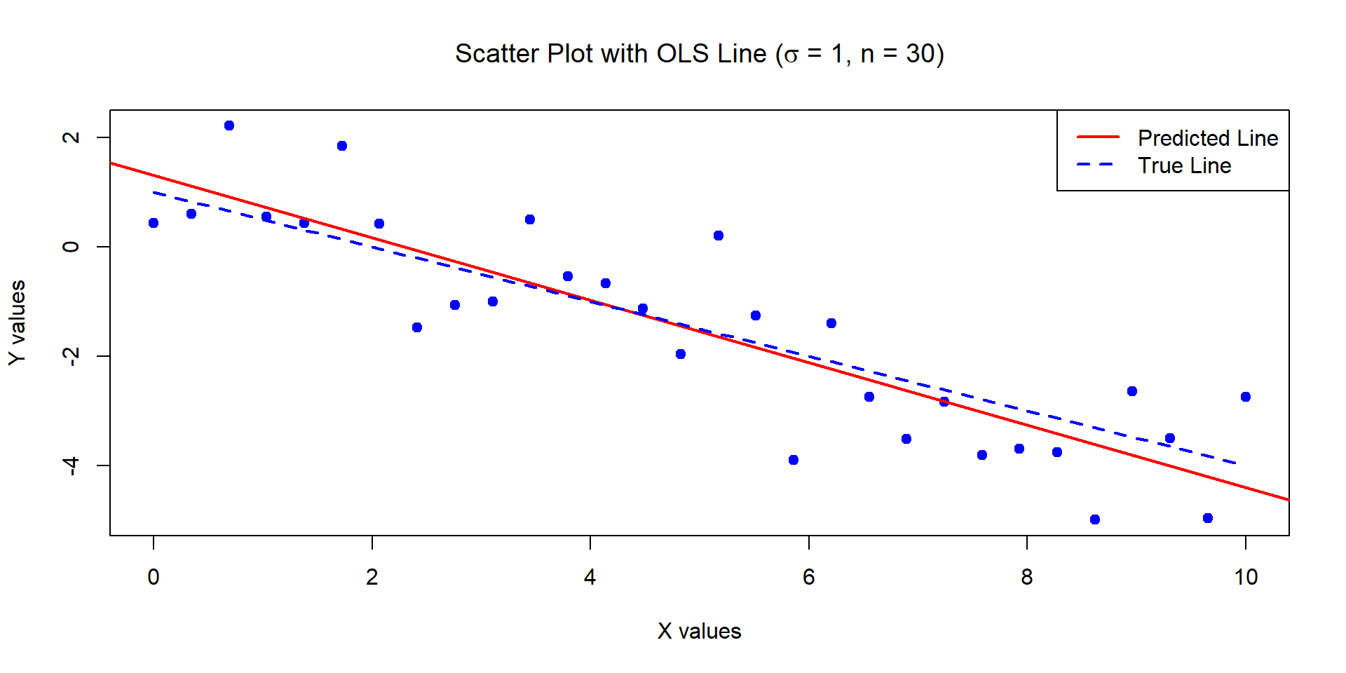
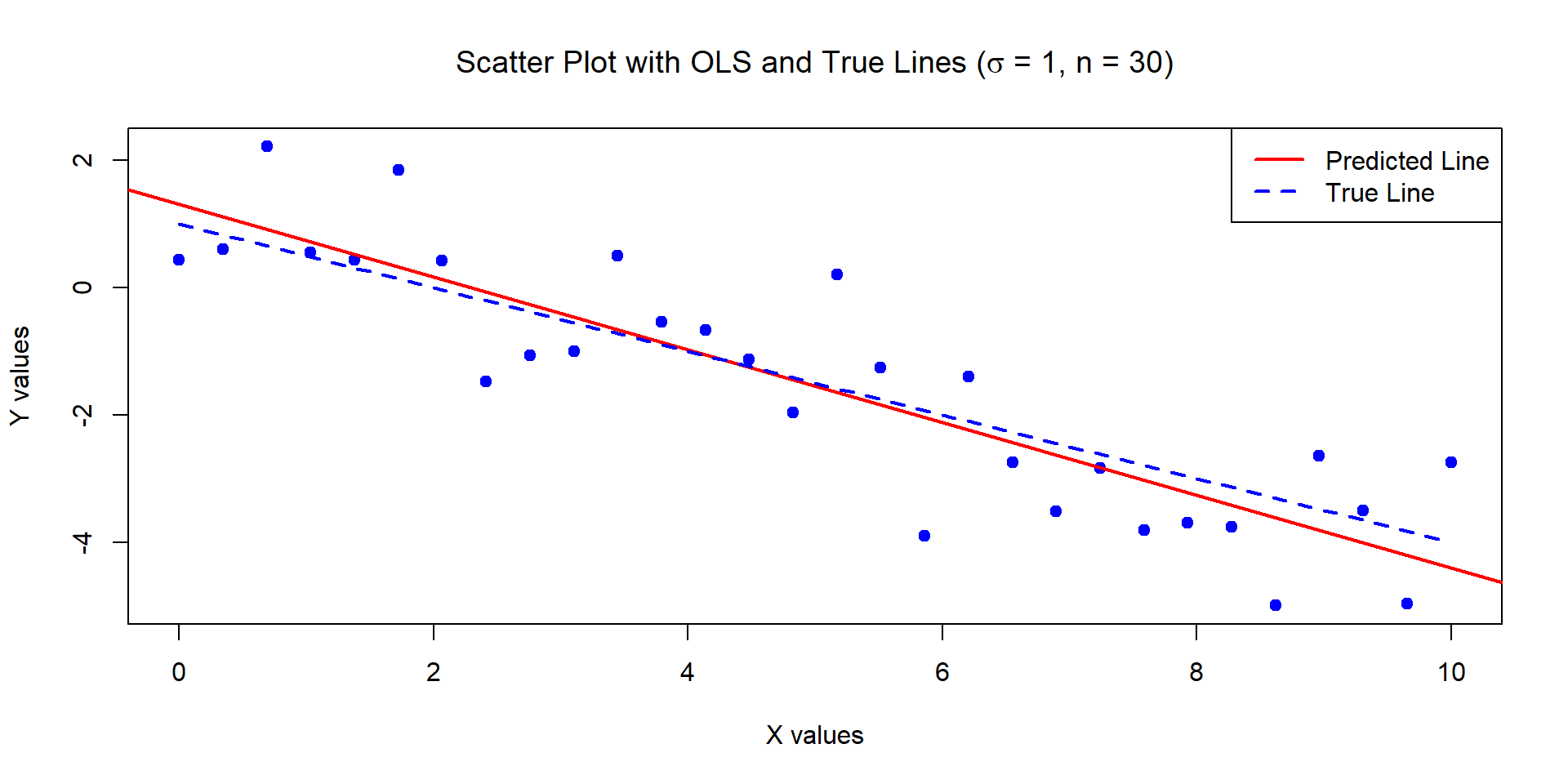
Example 1
The below data was generated by Y = 1 - 0.5\times X + \epsilon where X \sim U[0,10] and \epsilon \sim N(0,1) with n = 30.
Estimates of Beta_0 and Beta_1:
 1.309629 -0.5713465
Standard error of the estimates:
 0.346858 0.05956626
![]()
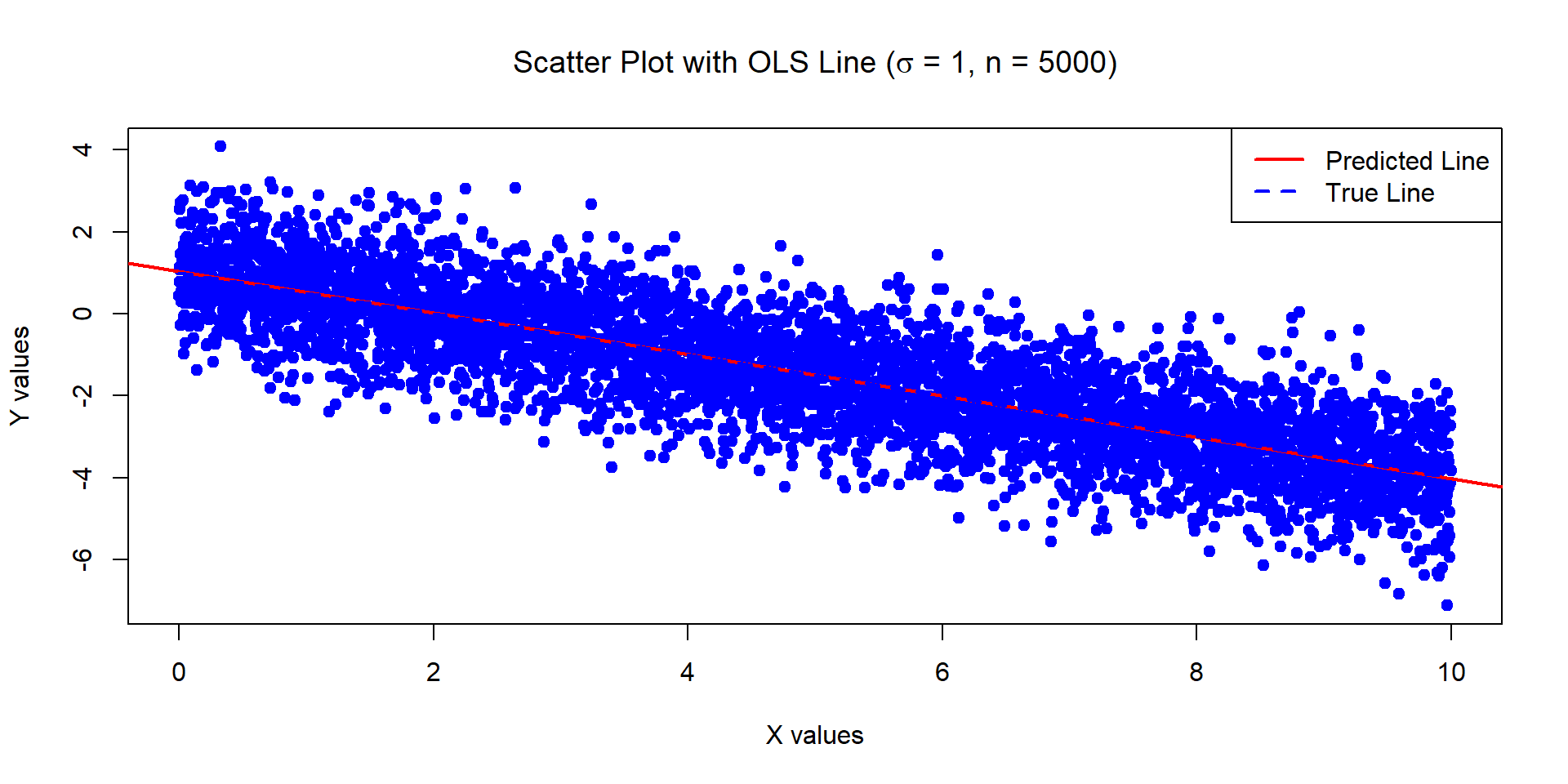
Example 2
The below data was generated by Y = 1 - 0.5\times X + \epsilon where X \sim U[0,10] and \epsilon \sim N(0,1) with n = 5000.
Estimates of Beta_0 and Beta_1:
 1.028116 -0.5057372
Standard error of the estimates:
 0.02812541 0.00487122
![]()
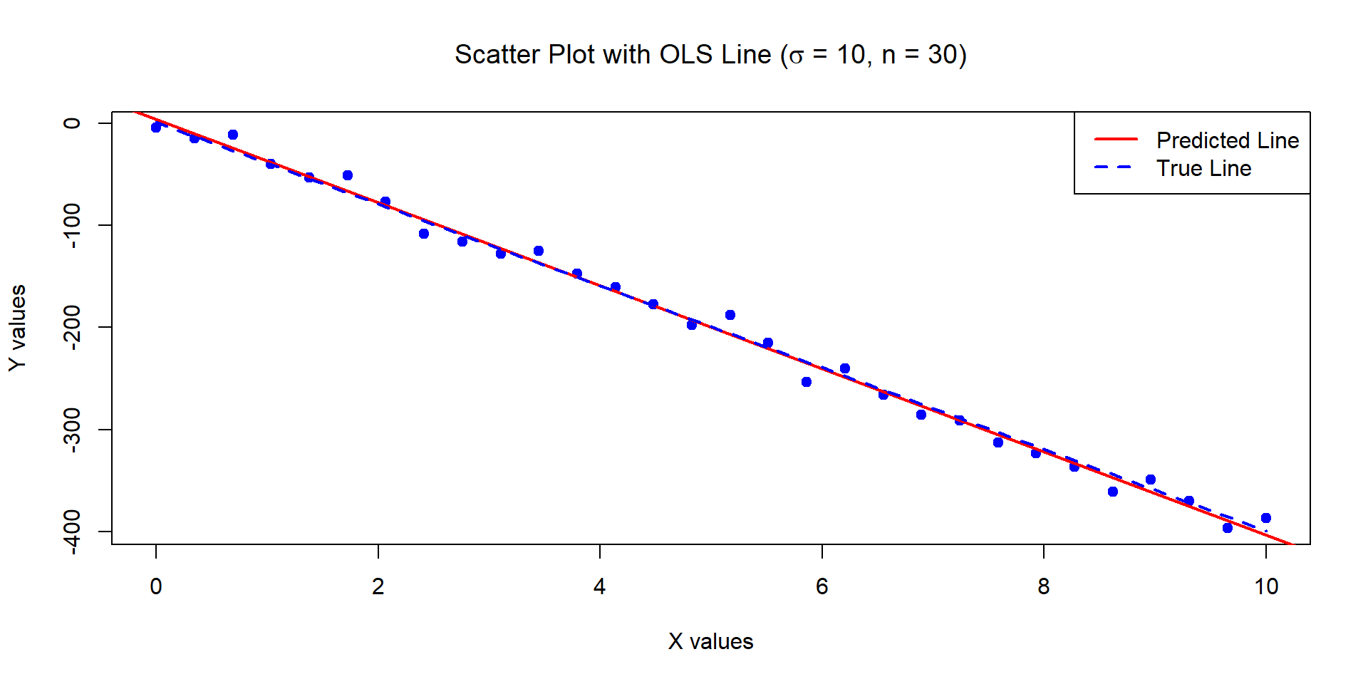
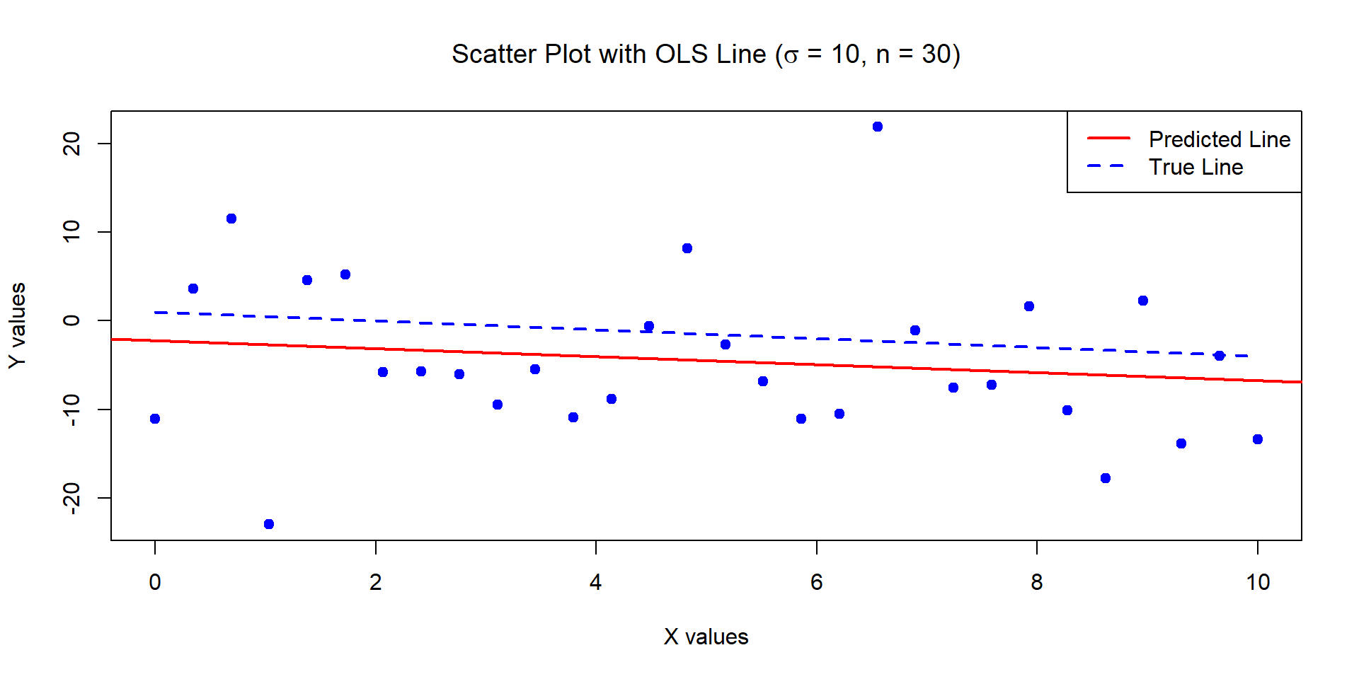
Example 3
The below data was generated by Y = 1 - 0.5\times X + \epsilon where X \sim U[0,10] and \epsilon \sim N(0, \sigma^2=100) with n = 30.
Estimates of Beta_0 and Beta_1:
 -2.19991 -0.4528679
Standard error of the estimates:
 3.272989 0.5620736
![]()
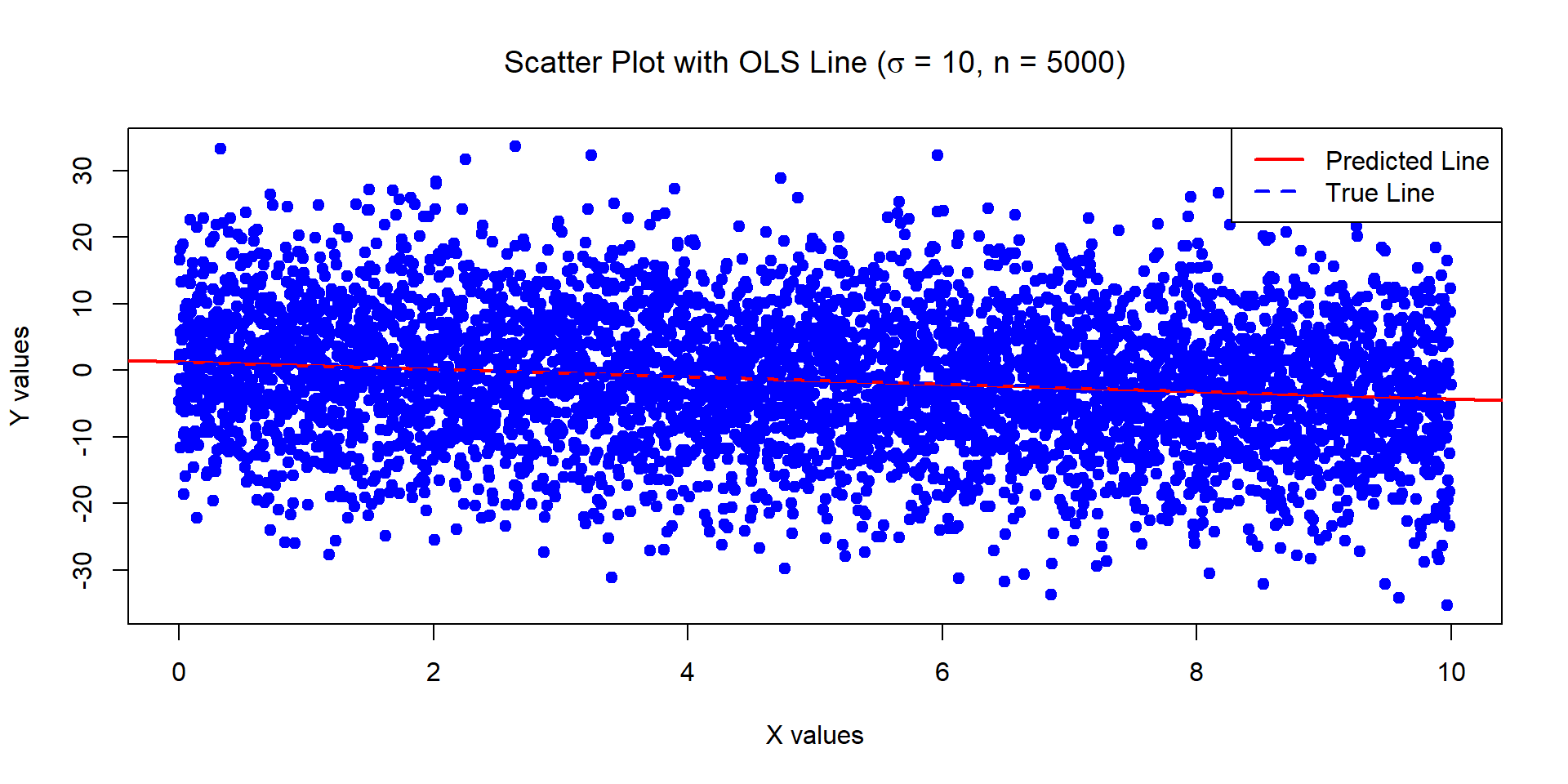
Example 4
The below data was generated by Y = 1 - 0.5\times X + \epsilon where X \sim U[0,10] and \epsilon \sim N(0, \sigma^2=100) with n = 5000.
Estimates of Beta_0 and Beta_1:
 1.281162 -0.5573716
Standard error of the estimates:
 0.2812541 0.0487122
![]()
Example 5
The below data was generated by Y = 1 - 40\times X + \epsilon where X \sim U[0,10] and \epsilon \sim N(0,100) with n = 30.
Estimates of Beta_0 and Beta_1:
 4.096286 -40.71346
Standard error of the estimates:
 3.46858 0.5956626
![]()
Assessing the models
- How do we know which models to “trust”?
- Estimates for examples 1, 2 and 4 seem good (parameter estimates quite close to true values, and low standard errors).
- We are less confident in example 3 (higher standard errors).
- Discussion question: what do you think of the model in example 5? Are you worried about the standard errors?
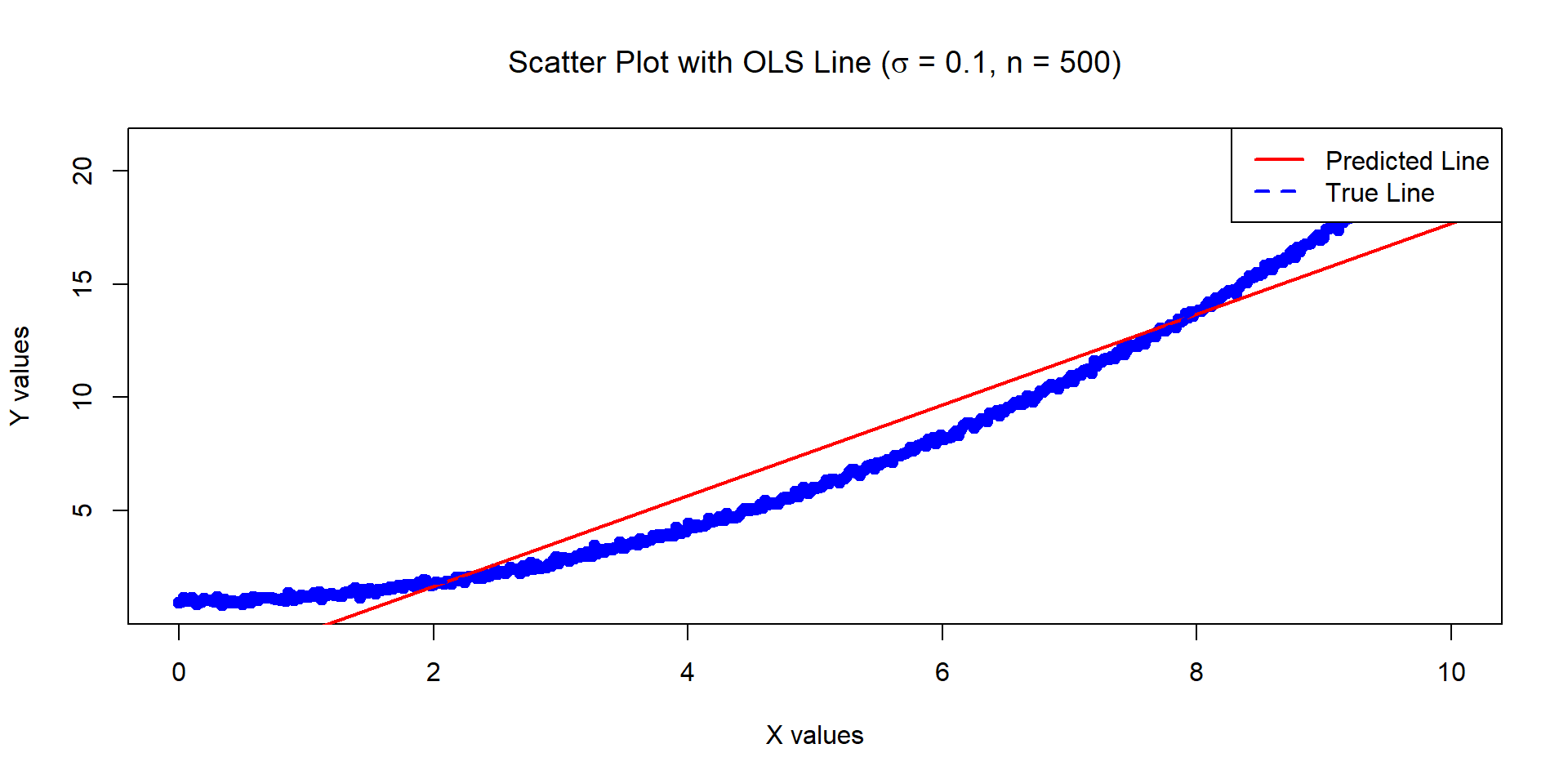
- Consider the next example, it has low standard errors but it doesn’t look ‘right’… why is that?
Example 6
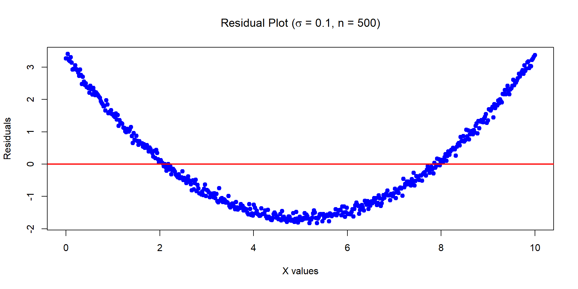
The below data was generated by Y = 1 + 0.2 \times X^2 + \epsilon where X \sim U[0,10] and \epsilon \sim N(0, \sigma^2=0.01) with n = 500.
Estimates of Beta_0 and Beta_1:
 -2.32809 2.000979
Variances of the estimates:
 0.01808525 0.0005420144
![]()
Assessing the Accuracy I
- How to assess the accuracy of the coefficient estimates? In particular, consider the following questions:
- What are the confidence intervals for {\beta}_0 and {\beta}_1?
- How to test the null hypothesis that there is no relationship between X and Y?
- How to test if the influence of the predictor variable (X) on the response variable (Y) is larger/smaller than some value?
For inference (e.g., confidence intervals, hypothesis tests), we need the strong assumptions!
Assessing the Accuracy of the Coefficient Estimates - Confidence Intervals
Using the strong assumptions, 100\left( 1-\alpha \right) \% confidence intervals (CI) for \beta_1 and \beta_0 are given by:
\hat{\beta}_1\pm t_{1-\alpha /2,n-2}\cdot \underbrace{\dfrac{s}{\sqrt{S_{xx}}}}_{\hat{SE}(\hat{\beta}_1)}
\hat{\beta}_0\pm t_{1-\alpha /2,n-2}\cdot \underbrace{s\sqrt{\frac{1}{n}+\frac{\overline{x}^2}{S_{xx}}}}_{\hat{SE}(\hat{\beta}_0)}
See rationale slide.
Assessing the Accuracy of the Coefficient Estimates - Inference on the slope
We can test whether the predictor has any influence on the response (or if the influence is larger/smaller than some value).
For testing the hypothesis H_{0}:\beta_1 =\widetilde{\beta}_1 \quad\text{vs}\quad H_{1}:\beta_1 \neq \widetilde{\beta}_1, (where \widetilde{\beta}_1 is any constant) we use the test statistic: t(\hat{\beta}_1) = \dfrac{\hat{\beta}_1-\widetilde{\beta}_1}{\hat{SE}(\hat{\beta_1})}=\dfrac{\hat{\beta}_1-\widetilde{\beta}_1}{\left( s\left/ \sqrt{S_{xx}}\right. \right)} which has a t_{n-2} distribution under H_0 (see rationale slide).
The construction of the hypothesis test is the same for \beta_0.
Assessing the Accuracy of the Coefficient Estimates - Inference on the slope
The decision rules under various alternative hypotheses are summarized below.
Decision Making Procedures for Testing H_{0}:\beta_1=\widetilde{\beta}_1
| \beta_1 \neq \widetilde{\beta}_1 |
\left\vert t\left( \hat{\beta}_1\right) \right\vert >t_{1-\alpha /2,n-2} |
| \beta_1 >\widetilde{\beta}_1 |
t\left( \hat{\beta}_1\right)>t_{1-\alpha ,n-2} |
| \beta_1 <\widetilde{\beta}_1 |
t\left( \hat{\beta}_1\right)<-t_{1-\alpha ,n-2} |
- Note we are usually interested in testing H_0: \beta_1 = 0 vs. H_1: \beta_1 \neq 0, as this informs us whether our \beta_1 is significantly different from 0. I.e., the predictor has some influence on the response.
- Similar construction to test the significance of \beta_0.
Example 1 - Hypothesis testing
The below data was generated by Y = 1 - 0.5\times X + \epsilon where X \sim U[0,10] and \epsilon \sim N(0,1) with n = 30.
Call:
lm(formula = Y ~ X)

Residuals:
    Min      1Q  Median      3Q     Max
-1.8580 -0.7026 -0.1236  0.5634  1.8463

Coefficients:
            Estimate Std. Error t value Pr(>|t|)
(Intercept)  1.30963    0.34686   3.776 0.000764 ***
X           -0.57135    0.05957  -9.592  2.4e-10 ***
---
Signif. codes:  0 '***' 0.001 '**' 0.01 '*' 0.05 '.' 0.1 ' ' 1

Residual standard error: 0.9738 on 28 degrees of freedom
Multiple R-squared:  0.7667,    Adjusted R-squared:  0.7583
F-statistic:    92 on 1 and 28 DF,  p-value: 2.396e-10
![]()
Example 2 - Hypothesis testing
The below data was generated by Y = 1 - 0.5\times X + \epsilon where X \sim U[0,10] and \epsilon \sim N(0,1) with n = 5000.
Call:
lm(formula = Y ~ X)

Residuals:
    Min      1Q  Median      3Q     Max
-3.1179 -0.6551 -0.0087  0.6655  3.4684

Coefficients:
             Estimate Std. Error t value Pr(>|t|)
(Intercept)  1.028116   0.028125   36.55   <2e-16 ***
X           -0.505737   0.004871 -103.82   <2e-16 ***
---
Signif. codes:  0 '***' 0.001 '**' 0.01 '*' 0.05 '.' 0.1 ' ' 1

Residual standard error: 0.9945 on 4998 degrees of freedom
Multiple R-squared:  0.6832,    Adjusted R-squared:  0.6831
F-statistic: 1.078e+04 on 1 and 4998 DF,  p-value: < 2.2e-16
![]()
Example 3 - Hypothesis testing
The below data was generated by Y = 1 - 0.5\times X + \epsilon where X \sim U[0,10] and \epsilon \sim N(0,100) with n = 30.
Call:
lm(formula = Y ~ X)

Residuals:
    Min      1Q  Median      3Q     Max
-20.306  -5.751  -2.109   5.522  27.049

Coefficients:
            Estimate Std. Error t value Pr(>|t|)
(Intercept)  -2.1999     3.2730  -0.672    0.507
X            -0.4529     0.5621  -0.806    0.427

Residual standard error: 9.189 on 28 degrees of freedom
Multiple R-squared:  0.02266,   Adjusted R-squared:  -0.01225
F-statistic: 0.6492 on 1 and 28 DF,  p-value: 0.4272
![]()
Example 4 - Hypothesis testing
The below data was generated by Y = 1 - 0.5\times X + \epsilon where X \sim U[0,10] and \epsilon \sim N(0,100) with n = 5000.
Call:
lm(formula = Y ~ X)

Residuals:
    Min      1Q  Median      3Q     Max
-31.179  -6.551  -0.087   6.655  34.684

Coefficients:
            Estimate Std. Error t value Pr(>|t|)
(Intercept)  1.28116    0.28125   4.555 5.36e-06 ***
X           -0.55737    0.04871 -11.442  < 2e-16 ***
---
Signif. codes:  0 '***' 0.001 '**' 0.01 '*' 0.05 '.' 0.1 ' ' 1

Residual standard error: 9.945 on 4998 degrees of freedom
Multiple R-squared:  0.02553,   Adjusted R-squared:  0.02533
F-statistic: 130.9 on 1 and 4998 DF,  p-value: < 2.2e-16
![]()
Example 5 - Hypothesis testing
The below data was generated by Y = 1 - 40\times X + \epsilon where X \sim U[0,10] and \epsilon \sim N(0,100) with n = 30.
Call:
lm(formula = Y ~ X)

Residuals:
    Min      1Q  Median      3Q     Max
-18.580  -7.026  -1.236   5.634  18.463

Coefficients:
            Estimate Std. Error t value Pr(>|t|)
(Intercept)   4.0963     3.4686   1.181    0.248
X           -40.7135     0.5957 -68.350   <2e-16 ***
---
Signif. codes:  0 '***' 0.001 '**' 0.01 '*' 0.05 '.' 0.1 ' ' 1

Residual standard error: 9.738 on 28 degrees of freedom
Multiple R-squared:  0.994, Adjusted R-squared:  0.9938
F-statistic:  4672 on 1 and 28 DF,  p-value: < 2.2e-16
![]()
Example 6 - Hypothesis testing
The below data was generated by Y = 1 + 0.2 \times X^2 + \epsilon where X \sim U[0,10] and \epsilon \sim N(0,0.01) with n = 500.
Call:
lm(formula = Y ~ X)

Residuals:
    Min      1Q  Median      3Q     Max
-1.8282 -1.3467 -0.4217  1.1207  3.4041

Coefficients:
            Estimate Std. Error t value Pr(>|t|)
(Intercept) -2.32809    0.13448  -17.31   <2e-16 ***
X            2.00098    0.02328   85.95   <2e-16 ***
---
Signif. codes:  0 '***' 0.001 '**' 0.01 '*' 0.05 '.' 0.1 ' ' 1

Residual standard error: 1.506 on 498 degrees of freedom
Multiple R-squared:  0.9368,    Adjusted R-squared:  0.9367
F-statistic:  7387 on 1 and 498 DF,  p-value: < 2.2e-16
![]()
Summary of hypothesis tests
Below is the summary of the hypothesis tests for whether the \beta_j are statistically different from 0 for the six examples, at a 5% level.
| \beta_0 |
Y |
Y |
N |
Y |
N |
Y |
| \beta_1 |
Y |
Y |
N |
Y |
Y |
Y |
Does that mean the models that are significant at 5% for both \beta_0 and \beta_1 are equivalently ‘good’ models?
- No!
- Model 5 looks like it would have the most “predictive power”, even though \beta_0 is not significant.
- Model 6 has significant estimates, but is misspecified (clearly the underlying relationship is not linear).
Assessing the accuracy of the model
We have the following so far:
- Data plotting with model predictions overlayed.
- Estimates of a linear model coefficients \hat{\beta}_0 and \hat{\beta}_1.
- Standard errors and hypothesis tests on the coefficients.
We now discuss how to assess whether a model is ‘good’ / ‘accurate’?
Assessing the accuracy of the model
Partitioning the variability is used to assess how well the linear model explains the trend in data:
\underset{\text{total deviation}}{\underbrace{y_{i}-\overline{y}}}=\underset{\text{unexplained deviation}}{\underbrace{\left( y_{i}-\hat{y}_{i}\right) }}+\underset{\text{explained deviation}}{\underbrace{\left( \hat{y}_{i}-\overline{y}\right). }}
We can show (see Lab questions) that :
\underset{\text{TSS}}{\underbrace{\overset{n}{\underset{i=1}{\sum }}\left( y_{i}-\overline{y}\right) ^{2}}}=\underset{\text{RSS}}{\underbrace{\overset{n}{\underset{i=1}{\sum }}\left( y_{i}-\hat{y}_{i}\right) ^{2}}}+\underset{\text{MSS}}{\underbrace{\overset{n}{\underset{i=1}{\sum }}\left( \hat{y}_{i}-\overline{y}\right) ^{2}}},
- TSS: total sum of squares;
- RSS: residual sum of squares;
- MSS: model sum of squares (also known as “explained sum of squares”, ESS, but here we stick to MSS).
Assessing the accuracy of the model
How to interpret these sums of squares:
- TSS is the total variability in the y_i values (note how it’s proportional to the sample variance of Y);
- MSS is the variability in the y_i that is “explained” or “captured” by our model (i.e., by our knowledge that X is predicting Y).
- RSS is the variability that remains “unexplained”, even after capturing the effect of X on Y.
This partitioning of the variability is used in “ANOVA tables”:
| Regression |
\text{MSS}= \sum_{i=1}^{n} (\hat{y_i} - \bar{y})^2 |
\text{DFM} = 1 |
\frac{\text{MSS}}{\text{DFM}} |
\frac{\text{MSS}/\text{DFM}}{\text{RSS}/\text{DFE}} |
| Error |
\text{RSS}= \sum_{i=1}^{n} (y_i - \hat{y_i})^2 |
\text{DFE} = n-2 |
\frac{\text{RSS}}{\text{DFE}} |
|
| Total |
\text{TSS} = \sum_{i=1}^{n} (y_i - \bar{y})^2 |
\text{DFT} = n-1 |
\frac{\text{TSS}}{\text{DFT}} |
|
Assessing the accuracy of the model: R^2
- We now define an important metric to quantify how “good” our model is: R^2.
- It has several equivalent definitions, but a simple one is as follows:
R^2 = \frac{\text{MSS}}{\text{TSS}} = 1 - \frac{\text{RSS}}{\text{TSS}}.
- R^2 is interpreted as the “proportion of variability in Y that can be explained using X” (James et al., 2021).
Alernative definition of R^2
- It is not too hard to show (see Lab) that:
\begin{aligned}
\text{MSS} = \hat{\beta}_1 S_{xy}.
\end{aligned}
Hence, recalling that \hat{\beta}_1=S_{xy}/S_{xx}, we obtain:
\begin{aligned}
R^2= \frac{\text{MSS}}{\text{TSS}} = \left(\frac{S_{xy}^2}{S_{xx}} \right) \cdot \frac{1}{S_{yy}} = \left(\frac{S_{xy}}{\sqrt{S_{xx}\cdot S_{yy}}} \right)^2.
\end{aligned}
- This shows that, in simple linear regression, R^2 is simply the square of the good old sample correlation between X and Y.
- Hence, we know it takes values between 0 and 1.
Summary of R^2 from the six examples
Below is a table of the R^2 for all of the six examples:
| R^2 |
0.77 |
0.68 |
0.02 |
0.03 |
0.99 |
0.94 |
- The R^2 for {1, 2}, and {3, 4} are similar (as expected, since we only changed n).
- Example 5 has the highested R^2 despite having an insignificant \beta_0.
- Example 6 has a surprisingly high R^2 (despite the data being non-linear). But Example 6 does not satisfy the assumptions of our model, so the results are dubious. (More on this later)
- Careful: a single number can’t give you the whole story!
Multiple Linear Regression
Multiple Linear Regression
Diagnostics in MLR: ANOVA, R^2, F-test
Potential issues with Linear Regression
Overview
- We extend the simple linear regression model to include “p” predictors: Y = \beta_0 + \beta_1 X_1 + \beta_2 X_2 + \cdots + \beta_p X_p + \epsilon
- The capital letters Y and X_1,\ldots X_p mean we conceptualise those quantities as “random variables”.
- The response Y is still a linear function of individual predictors.
- \beta_j is the average effect on Y (increase if positive, decrease if negative) of a one unit increase in X_j (holding all other X_{k}, k \neq j variables fixed).
- Instead of fitting a line, we are now fitting a (hyper-)plane.
Vector notation
- For an observed sample of size n, (y_{1}, x_{11}, x_{12}, ..., x_{1p}), ..., (y_{n}, x_{n1},...,x_{np}), we denote our n responses \bm{y} = (y_1, \ldots, y_n)^{\top}.
- For the predictors, we denote x_{ij} the jth predictor of observation i (this is a scalar).
- We denote \bm{x}_j = (x_{1j}, x_{2j}, \ldots, x_{nj})^{\top} the n observed values of predictor j.
- Hence, our model for all observations can be written \bm{y} = \beta_0 \bm{1} + \beta_1 \bm{x}_1 + \beta_2 \bm{x}_2 + \ldots + \beta_p \bm{x}_p + \bm{\epsilon}. where \bm{1} is a column vector of 1’s (of size n) and \bm{\epsilon} is defined as in simple linear regression.
Advertising Example
\texttt{sales} \approx \beta_0 + \beta_1 \times \texttt{TV}+ \beta_2 \times \texttt{radio}
![]()
Matrix notation
- With matrix notation, we can write the model in an even more compact manner.
- Let \bm{\beta} = (\beta_0, \beta_1, \ldots, \beta_p)^{\top} be a column vector (of size p+1).
- Let \bm{X} be the design matrix, of size n \times (p+1), defined as
\bm{X}=\left[
\begin{array}{ccccc}
1 & x_{11} & x_{12} & \ldots & x_{1p} \\
1 & x_{21} & x_{22} & \ldots & x_{2p} \\
\vdots & \vdots & \vdots & \ddots & \vdots \\
1 & x_{n1} & x_{n2} & \ldots & x_{np}
\end{array}
\right]
- Then, our linear regression model can be written as \bm{y} = \bm{X}\bm{\beta} + \bm{\epsilon}.
- Make sure you agree all the dimensions make sense.
- Do you see that simple linear regression can be recovered from this notation?
Assumptions on the error terms
The asssumptions made about the errors are as in simple linear regression:
The error terms \epsilon_{i} satisfy the following:
\begin{aligned}
\begin{array}{rll}
\mathbb{E}[ \epsilon _{i}|\bm{X}] =&0, &\text{ for }i=1,2,\ldots,n; \\
\text{Var}( \epsilon _{i}|\bm{X}) =&\sigma ^{2}, &\text{ for }i=1,2,\ldots,n;\\
\text{Cov}( \epsilon _{i},\epsilon _{j}|\bm{X})=&0, &\text{ for all }i\neq j.
\end{array}
\end{aligned}
In words, the errors have zero means, common variance, and are uncorrelated. In matrix form, we have:
\begin{aligned}
\mathbb{E}\left[ \bm{\epsilon} | \bm{X}\right] = \bm{0}; \qquad
\text{Cov}\left( \bm{\epsilon} | \bm{X} \right) =\sigma^{2} I_n,
\end{aligned}
where I_n is the n\times n identity matrix.
- Strong Assumptions: \epsilon_{i}|\bm{X} \stackrel{\text{i.i.d}}{\sim} \mathcal{N}(0, \sigma^2).
Least Squares Estimates (LSE)
- Same least squares approach as in Simple Linear Regression: we pick the estimates \hat{\beta}_0, \ldots, \hat{\beta}_p that minimise the residual sum of squares (RSS):
\begin{aligned}
\text{RSS} &= \sum_{i=1}^{n}\left(y_{i}-\hat{y}_{i}\right)^{2}=\sum_{i=1}^{n}\left( y_{i}-\hat{\beta} _{0}-\hat{\beta} _{1}x_{i1}- \ldots -\hat{\beta} _{p}x_{ip}\right)^{2} =\sum_{i=1}^{n} \hat{\epsilon}_{i}^{2} \\
&= \left( \bm{y} - \bm{X} \hat{\bm{\beta}} \right)^{\top}\left(\bm{y}-\bm{X}\hat{\bm{\beta}}\right).
\end{aligned}
- If \left(\bm{X}^{\top}\bm{X}\right)^{-1} exists, it can be shown that the solution is given by: \hat{\bm{\beta}}=\left(\bm{X}^{\top} \bm{X} \right)^{-1} \bm{X}^{\top} \bm{y}.
- The corresponding vector of fitted (or predicted) values is \bm{\hat{y}}=\bm{X}\bm{\hat{\beta}}.
Least Squares Estimates (LSE) - Properties
Under the weak assumptions we have unbiased estimators:
- The least squares estimators are unbiased: \mathbb{E}[ \hat{\beta}_j] = \beta_j, \; \forall j.
- The variance-covariance matrix of the least squares estimators is: \text{Var}(\hat{\bm{\beta}}) = \sigma^{2}\times \left(\bm{X}^{\top}\bm{X} \right)^{-1}
- An unbiased estimator of \sigma^{2} is: s^{2}=\dfrac{\text{RSS}}{n-p-1}, where p+1 is the total number of “\beta” parameters estimated.
- Under the strong assumptions, each \hat{\beta}_j is normally distributed. See details in slide.
Potential issues with Linear Regression
Multiple Linear Regression
Diagnostics in MLR: ANOVA, R^2, F-test
Potential issues with Linear Regression
Potential issues
- When fitting Linear Regression models, we are making strong assumptions about the data. If those assumptions are (substantially) incorrect, then the results from our models (inference, predictions) will be dubious.
- Specifically, we are assuming that:
- The relationships between the predictors and response are linear and additive;
- Errors have mean 0 and don’t dependent on predictors.
- Errors are homoskedastic (have constant variance) and their variance doesn’t dependent on predictors.
- Errors are uncorrelated;
- In the case of the “strong assumptions” (used for CI/statistical tests), errors are normally distributed.
Recall Example 6 - The problems
Recall the below data was generated by Y = 1 + 0.2 \times X^2 + \epsilon where X \sim U[0,10] and \epsilon \sim N(0, \sigma^2=0.01) with n = 500.
Mean of the residuals: -1.431303e-16
![]()
- Very strong pattern (“dependence”) between residuals and predictor: indicates our model is not appropriate.
Potential issues
- Non-linearity of the response-predictor relationships
- Correlation of error terms
- Non-constant variance of error terms
- Outliers
- High-leverage points
- Collinearity
- Confounding effect (correlation does not imply causality!)
1. Non-linearities
Example: residuals vs fitted for MPG vs Horsepower:
![]()
LHS is a linear model. RHS is a quadratic model.
In this example, the quadratic model removes much of the pattern (more on this later).
2. Correlations in the error terms
- The assumption in the regression model is that the error terms are uncorrelated with each other.
- If they are correlated the standard errors of parameter estimates can be incorrect.
![]()
3. Non-constant variance of error terms
The following are two regression outputs for Y (LHS) and \ln Y (RHS)
![]()
In this example, the log transformation removed much of the heteroscedasticity.
4. Outliers
An outlier is a point for which the response “y_i” is far from the value predicted by the model (otherwise said, it has a large residual y_i - \hat{y}_i).
![]()
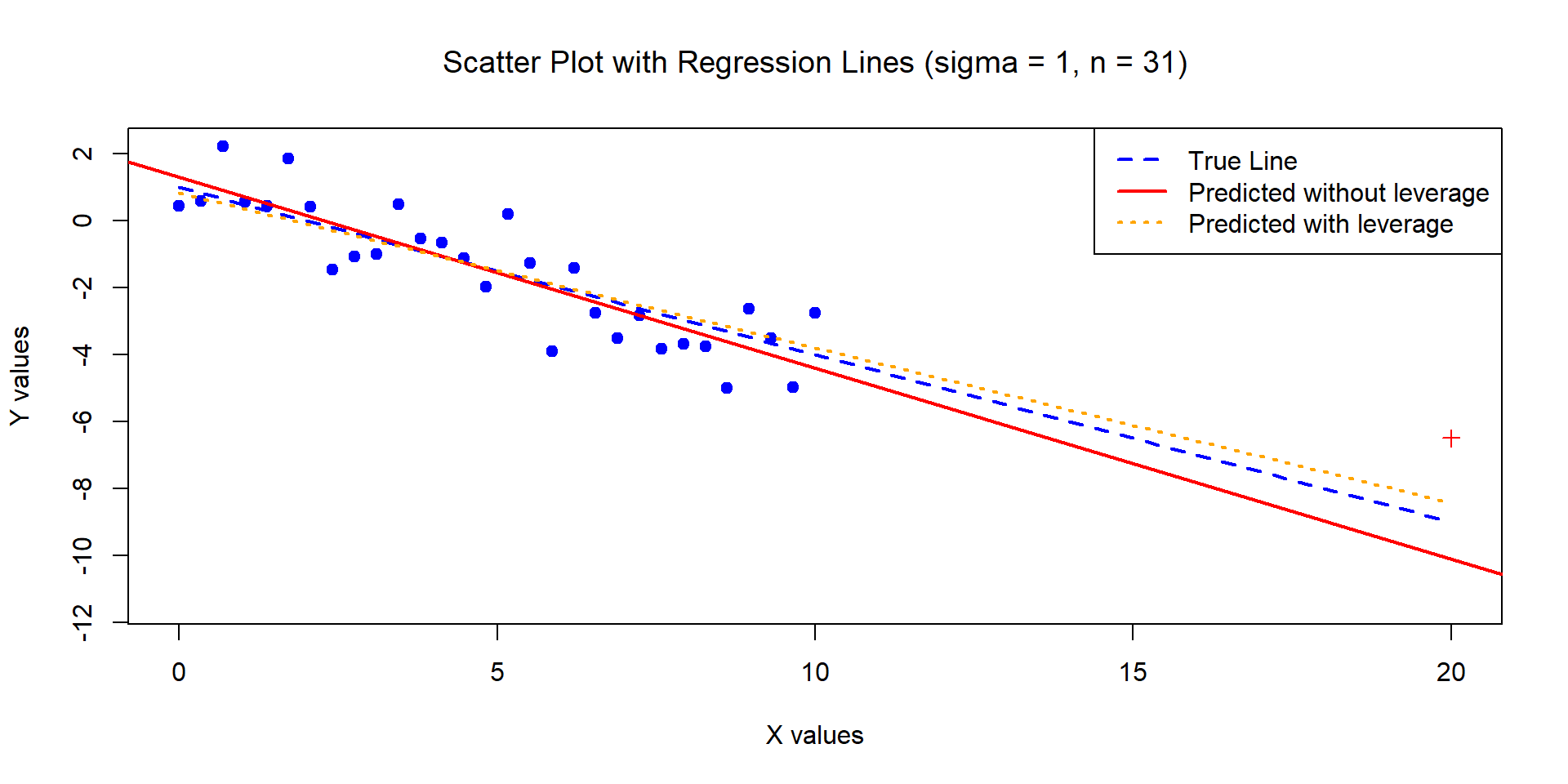
5. High-leverage points
- Observations with high leverage have an “unusual” value of their predictor(s).
- In the below data, point 20 is an outlier but not a leverage point, while 41 is a leverage point (and arguably an outlier too).
- Note that the red line was fitted with point 41, and the blue without point 41.
![]()
High-leverage points
- High leverage points are of concern because they have the potential to significantly affect the estimated regression line.
- We identify high leverage points via the hat matrix: \bm{H} = \bm{X}(\bm{X}^{\top}\bm{X})^{-1}\bm{X}^{\top}
- Note that \hat{y_{i}}=\sum^{n}_{j=1}h_{ij}y_j=h_{ii}y_i+\sum^{n}_{j\ne i}h_{ij}y_{j} so each prediction is a linear function of all observations, and h_{ii} = [\bm{H}]_{ii} is the weight of observation i on its own prediction.
- If h_{ii} > 2(p+1)/n, observation “i” is considered as having a high leverage.
High-leverage points (Example 1)
The below data was generated by Y = 1 - 0.5\times X + \epsilon where X \sim U[0,10] and \epsilon \sim N(0,1) with n = 30. We have added one high leverage point (made a red ‘+’ on the scatterplot).
- This point (y=-6.5,x=20) has a leverage value of 0.47 >> 4/31 (but you can’t really call it an outlier).
![]()
6. Collinearity
- Two or more predictors are closely related to each other (linearly dependent).
- High correlation between two predictors indicates collinearity.
- This is an issue because if columns of \bm{X} are linearly dependent, the matrix (\bm{X}^{\top}\bm{X}) is singular (non-invertible).
- Makes regression fitting tricky, because it increase the set of plausible coefficient values (\beta_j).
- Causes the SEs of the \beta_j coefficients to grow.
Collinearity makes optimisation harder
![]()
- Contour plots of the values of RSS as a function of the predictors’ coefficients.
Credit dataset used.
- Left:
balance regressed onto age and limit. Predictors have low collinearity.
- Right:
balance regressed onto rating and limit. Predictors have high collinearity.
- Black: coefficient estimate minimising RSS.
Multicollinearity
- More generally, a given predictor can be a linear function of several other predictors, and this is still a problem.
- We use the “variance inflation factor” (VIF): \text{VIF}(\hat{\beta}_j) = \frac{1}{1-R^2_{X_j|X_{-j}}}
- R^2_{X_j|X_{-j}} is the R^2 obtained from X_j being regressed onto all other predictors.
- Hence, it measures the strength of the linear relationship between the response variable (X_j) and all other predictors.
- The minimum VIF is 1 (high values are “bad”).
- Rule of thumb: >5 or >10 is considered high.
Multicollinearity example - Plot
The below data was generated by Y = 1 - 0.7\times X_1 + X_2 + \epsilon where \epsilon \sim N(0,1), X_1 \sim U[0,10], X_2 = 2X_1. Note n = 30.
Multicollinearity example - Summary and VIF
The below data was generated by Y = 1 - 0.7\times X_1 + X_2 + \epsilon where \epsilon \sim N(0,1) and X_1 \sim U[0,10], X_2 = 2X_1 + \varepsilon, where \varepsilon \sim N(0,10^{-8}) is a small quantity (so the fitting “works”). Note n=30.
Call:
lm(formula = Y ~ X1 + X2)

Residuals:
     Min       1Q   Median       3Q      Max
-2.32126 -0.46578  0.02207  0.54006  1.89817

Coefficients:
              Estimate Std. Error t value Pr(>|t|)
(Intercept)  5.192e-01  3.600e-01   1.442   0.1607
X1           5.958e+04  3.268e+04   1.823   0.0793 .
X2          -2.979e+04  1.634e+04  -1.823   0.0793 .
---
Signif. codes:  0 '***' 0.001 '**' 0.01 '*' 0.05 '.' 0.1 ' ' 1

Residual standard error: 0.8538 on 27 degrees of freedom
Multiple R-squared:  0.9614,    Adjusted R-squared:  0.9585
F-statistic: 335.9 on 2 and 27 DF,  p-value: < 2.2e-16
- High SE on the coefficient estimates, making them unreliable.
7. Confounding effects
- Lastly, we should mention that correlation does not imply causality!1
- Said otherwise, even if a predictor X is strongly significant in modelling a response Y via linear regression, it does not necessarily mean that X “causes” Y.
- C is a confounder (confounding variable) of the relation between X and Y if: C influences X and C influences Y.
- This induces a “relationship” between X and Y, but it does not mean that X causes Y (directly).
Confounding effects
- Example: the “age of a child” (X) would be correlated with their “aptitude for mathematics” (Y).
- But age alone does not “causes” a child to be better in mathematics, it is simply that:
- “time studying” \Rightarrow “age”
- “time studying” \Rightarrow “aptitude for mathematics”.
- Here, the confounder is “time studying”.
- If “time studying” cannot be measured, than “age” is a reasonable proxy… But it is not optimal, e.g., imagine a child you found in the jungle, or a child that never studies… they won’t be good at math even if they are older!
Confounding effects
How to correctly use/don’t use confounding variables?
- If a confounding variable is observable, add it to your model.
- If a confounding variable is unobservable, be careful with interpretation:
- in the presence of a confounder, action taken on the predictor alone will have no effect. E.g., “let’s not send our kid to school, they will grow old and automatically become good at maths”.
Appendices
Multiple Linear Regression
Diagnostics in MLR: ANOVA, R^2, F-test
Potential issues with Linear Regression
Appendix: Sum of squares
Recall from ACTL2131/ACTL5101, we have the following sum of squares:
\begin{aligned}
S_{xx} & =\sum_{i=1}^{n}(x_i-\overline{x})^2 &\implies s_x^2=\frac{S_{xx}}{n-1} \\
S_{yy} & =\sum_{i=1}^{n}(y_i-\overline{y})^2 &\implies s_y^2=\frac{S_{yy}}{n-1}\\
S_{xy} & =\sum_{i=1}^{n}(x_i-\overline{x})(y_i-\overline{y}) &\implies s_{xy}=\frac{S_{xy}}{n-1},
\end{aligned}
Here s_x^2, s_y^2 (and s_{xy}) denote sample (co-)variance.
Appendix: CI for \beta_1 and \beta_0
Rationale for \beta_1: Recall that \hat{\beta}_1 is unbiased and \text{Var}(\hat{\beta}_1)=\sigma^2/S_{xx}. However \sigma^2 is usually unknown, and estimated by s^2 so, under the strong assumptions, we have: \frac{\hat{\beta}_1-\beta_1 }{ s/ \sqrt{S_{xx}}} = \left.{\underset{\mathcal{N}(0,1)}{\underbrace{\frac{\hat{\beta}_1-\beta_1}{\sigma/ \sqrt{S_{xx}}}}}}\right/{\underset{\sqrt{\chi^2_{n-2}/(n-2)}}{\underbrace{\sqrt{\frac{\frac{(n-2)\cdot s^2}{\sigma^2}}{n-2}}}}} \sim t_{n-2} as \epsilon_i \overset{\text{i.i.d.}}{\sim} \mathcal{N}(0,\sigma^2) then \frac{(n-2)\cdot s^2}{\sigma^2} = \frac{\sum_{i=1}^{n}(y_i-\hat{\beta}_0-\hat{\beta}_1\cdot x_i)^2}{\sigma^2} \sim\chi^2_{{n}-2}.
Note: Why do we lose two degrees of freedom? Because we estimated two parameters!
Similar rationale for \beta_0.
Appendix: Statistical Properties of the Least Squares Estimates
- Under the strong assumptions of normality each component \hat{\beta}_{k} is normally distributed with mean and variance
\mathbb{E}[ \hat{\beta}_{k}] = \beta_k, \quad
\text{Var}( \hat{\beta}_{k}) = \sigma^2 \cdot c_{kk},
and covariance between \hat{\beta}_{k} and \hat{\beta}_{l}: \text{Cov}( \hat{\beta}_k, \hat{\beta}_l ) = \sigma^{2}\cdot c_{kl}, where c_{kk} is the \left( k+1\right)^{\text{th}} diagonal entry of the matrix {\mathbf{C}=}\left( \mathbf{X}^{\top}\mathbf{X}\right) ^{-1}.
The standard error of \hat{\beta}_{k} is estimated using \text{se}( \hat{\beta}_k ) = s\sqrt{c_{kk}}.
Simple linear regression: Assessing the Accuracy of the Predictions - Mean Response
Suppose x=x_{0} is a specified value of the out of sample regressor variable and we want to predict the corresponding Y value associated with it. The mean of Y is:
\begin{aligned}
\mathbb{E}[ Y \mid x_0 ] &= \mathbb{E}[ \beta_0 +\beta_1 x \mid x=x_0 ] \\
&= \beta_0 + \beta_1 x_0.
\end{aligned}
Our (unbiased) estimator for this mean (also the fitted value of y_0) is: \hat{y}_{0}=\hat{\beta}_0+\hat{\beta}_1x_{0}. The variance of this estimator is: \text{Var}( \hat{y}_0 ) = \left( \frac{1}{n} + \frac{(\overline{x}-x_0)^2}{S_{xx}}\right) \sigma ^{2} = \text{SE}(\hat{y}_0)^2
Proof: See Lab questions.
Simple linear regression: Assessing the Accuracy of the Predictions - Mean Response
Using the strong assumptions, the 100\left( 1-\alpha\right) \% confidence interval for \beta_0 +\beta_1 x_{0} (mean of Y) is:
\underbrace{\bigl(\hat{\beta}_0 + \hat{\beta}_1 x_0 \bigr)}_{\hat{y}_0} \pm t_{1-\alpha/2,n-2}\times {\underbrace{s\sqrt{ \dfrac{1}{n}+\dfrac{\left(\overline{x}-x_{0}\right) ^{2}}{S_{xx}}}}_{\hat{\text{SE}}(\hat{y}_0)}} ,
as we have
\hat{y}_{0} \sim \mathcal{N}( \beta_0 +\beta_1 x_{0}, \text{SE}(\hat{y}_0)^2
%={\left( \dfrac{1}{n}+\frac{\left( \overline{x}-x_{0}\right) ^{2}}{S_{xx}}\right)\sigma ^{2}}
)
and
\frac{\hat{y}_{0} - (\beta_0 +\beta_1 x_0)}{\hat{\text{SE}}(\hat{y}_0)}
%=\frac{\hat{y}_{0} - \left( \beta_0 +\beta_1 x_{0}\right)}{s\sqrt{\dfrac{1}{n}+\dfrac{\left( \overline{x}-x_{0}\right)^{2}}{S_{xx}} }}
\sim t(n-2).
Similar rationale to slide.
Simple linear regression: Assessing the Accuracy of the Predictions - Individual response
A prediction interval is a confidence interval for the actual value of a Y_i (not for its mean \beta_0 + \beta_1 x_i). We base our prediction of Y_i (given {X}=x_i) on: {\hat{y}}_i={\hat{\beta}}_0+{\hat{\beta}}_1x_i. The error in our prediction is:
\begin{aligned}
{Y}_i-{\hat{y}}_i=\beta_0+\beta_1x_i+{\epsilon}_i-{\hat{y}}_i=\mathbb{E}[{Y}|{X}=x_i]-{\hat{y}}_i+{\epsilon}_i.
\end{aligned}
with \mathbb{E}\left[{Y}_i-{\hat{y}}_i|{{X}}={x},{X}=x_i\right]=0 , \text{ and } \text{Var}({Y}_i-{\hat{y}}_i|{{X}}={x},{X}=x_i)=\sigma^2\bigl(1+{1\over n}+{(\overline{x} - x_i)^2\over S_{xx}}\bigr) .
Proof: See Lab questions.
Simple linear regression: Assessing the Accuracy of the Predictions - Individual response
A 100(1-\alpha)% prediction interval for {Y}_i, the value of {Y} at {X}=x_i, is given by:
\begin{aligned}
%&& {{\hat{y}}_i}\pm t_{1-\alpha/2,n-2}s\sqrt{1+\displaystyle{1\over n}+{(\overline{x} - x_i)^2\over S_{xx}}}\rule{140pt}{0pt}\\
%\equiv &&
{\underbrace{\hat{\beta}_0+\hat{\beta}_1x_i}_{\hat{y}_i}} \pm t_{1-\alpha/2,n-2}\cdot s\cdot\sqrt{1+\displaystyle{1\over n}+{(\overline{x} - x_i)^2\over S_{xx}}},
\end{aligned}
as
({Y}_i-{\hat{y}}_i|{\underline{X}}=\underline{x},{X}=x_i) \sim \mathcal{N}\Bigl(0, \sigma^2\bigl(1 + \frac1n + \frac{(\overline{x} - x_i)^2}{S_{xx}}\bigr)\Bigr) , \text{ and }
\frac{Y_i- \hat{y}_i}{s\sqrt{1 + \frac1n + \frac{(\overline{x} - x_i)^2}{S_{xx}}}} \sim t_{n-2}.