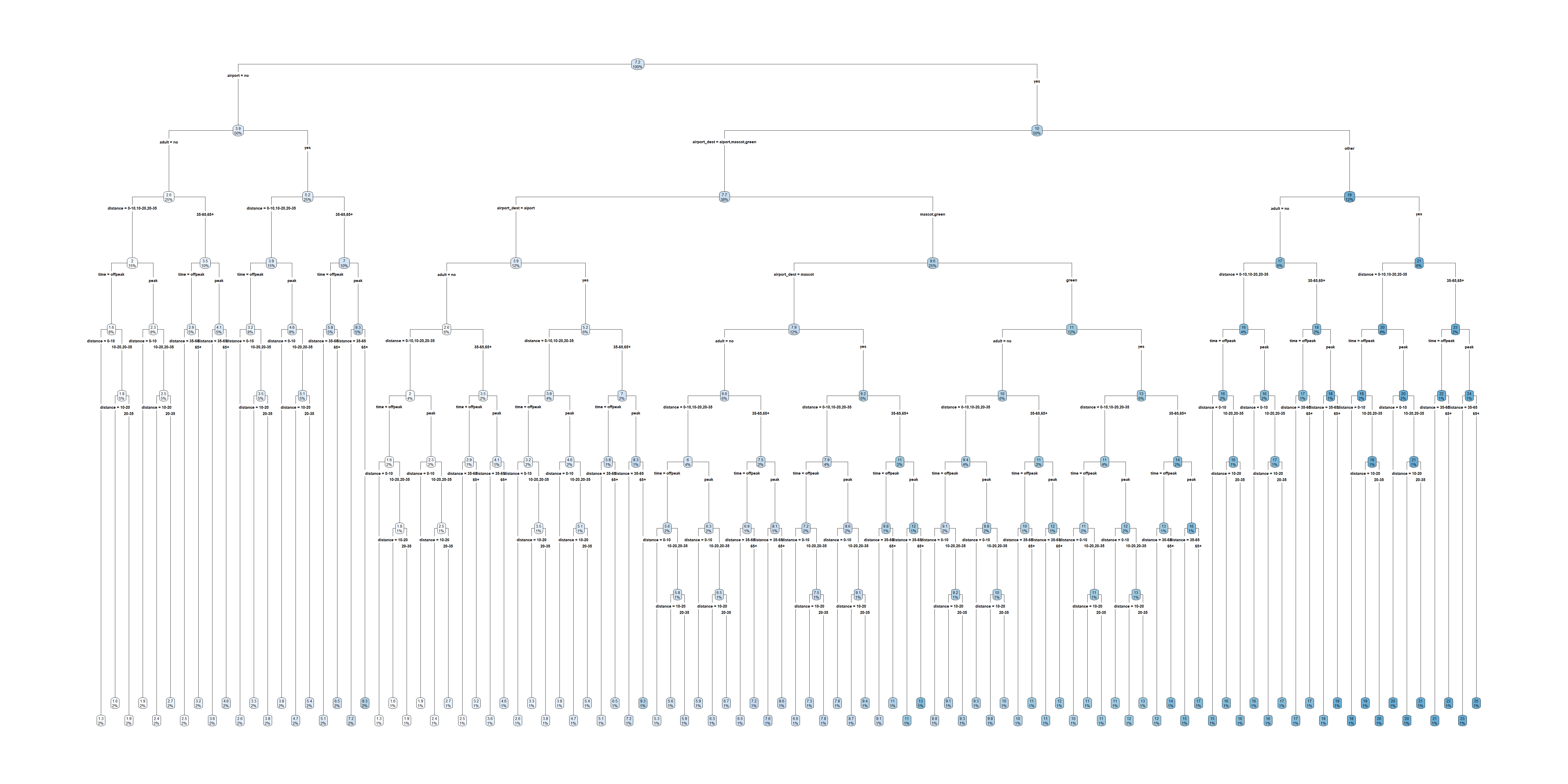
graph TB

    A{Is it peak hour?}
    A-->|Yes| B[Peak Hour]
    A-->|No| C[Off-Peak Hour]

    B--> D{Distance?}
    D-->|0 - 10 km| E[$3.79]
    D-->|10 - 20 km| F[$4.71]
    D-->|20 - 35 km| G[$5.42]
    D-->|35 - 65 km| H[$7.24]
    D-->|65+ km| I[$9.31]

    C--> J{Distance?}
    J-->|0 - 10 km| K[$2.65]
    J-->|10 - 20 km| L[$3.29]
    J-->|20 - 35 km| M[$3.79]
    J-->|35 - 65 km| N[$5.06]
    J-->|65+ km| O[$6.51]
Tree-Based Methods
ACTL3142 & ACTL5110 Statistical Machine Learning for Risk Applications
Trees in a nutshell
Decision trees are a simple, easy to interpret, and popular method for both regression and classification tasks. They can be used to make predictions, but also simply as “data exploration” to understand a data set better.
They make predictions by partitioning the predictor space into a number of simple regions, and making a constant prediction within each region. The set of splitting rules can be summarised in a tree. “Stand alone” tree models are rarely particularly accurate, but they form the basis for more accurate (and complex) methods like random forests and boosting.

Fit a basic tree
n= 263

node), split, n, deviance, yval
      * denotes terminal node

 1) root 263 207.153700 5.927222
   2) Years< 4.5 90  42.353170 5.106790
     4) Years< 3.5 62  23.008670 4.891812
       8) Hits< 114 43  17.145680 4.727386 *
       9) Hits>=114 19   2.069451 5.263932 *
     5) Years>=3.5 28  10.134390 5.582812 *
   3) Years>=4.5 173  72.705310 6.354036
     6) Hits< 117.5 90  28.093710 5.998380
      12) Years< 6.5 26   7.237690 5.688925 *
      13) Years>=6.5 64  17.354710 6.124096
        26) Hits< 50.5 12   2.689439 5.730017 *
        27) Hits>=50.5 52  12.371640 6.215037 *
     7) Hits>=117.5 83  20.883070 6.739687 *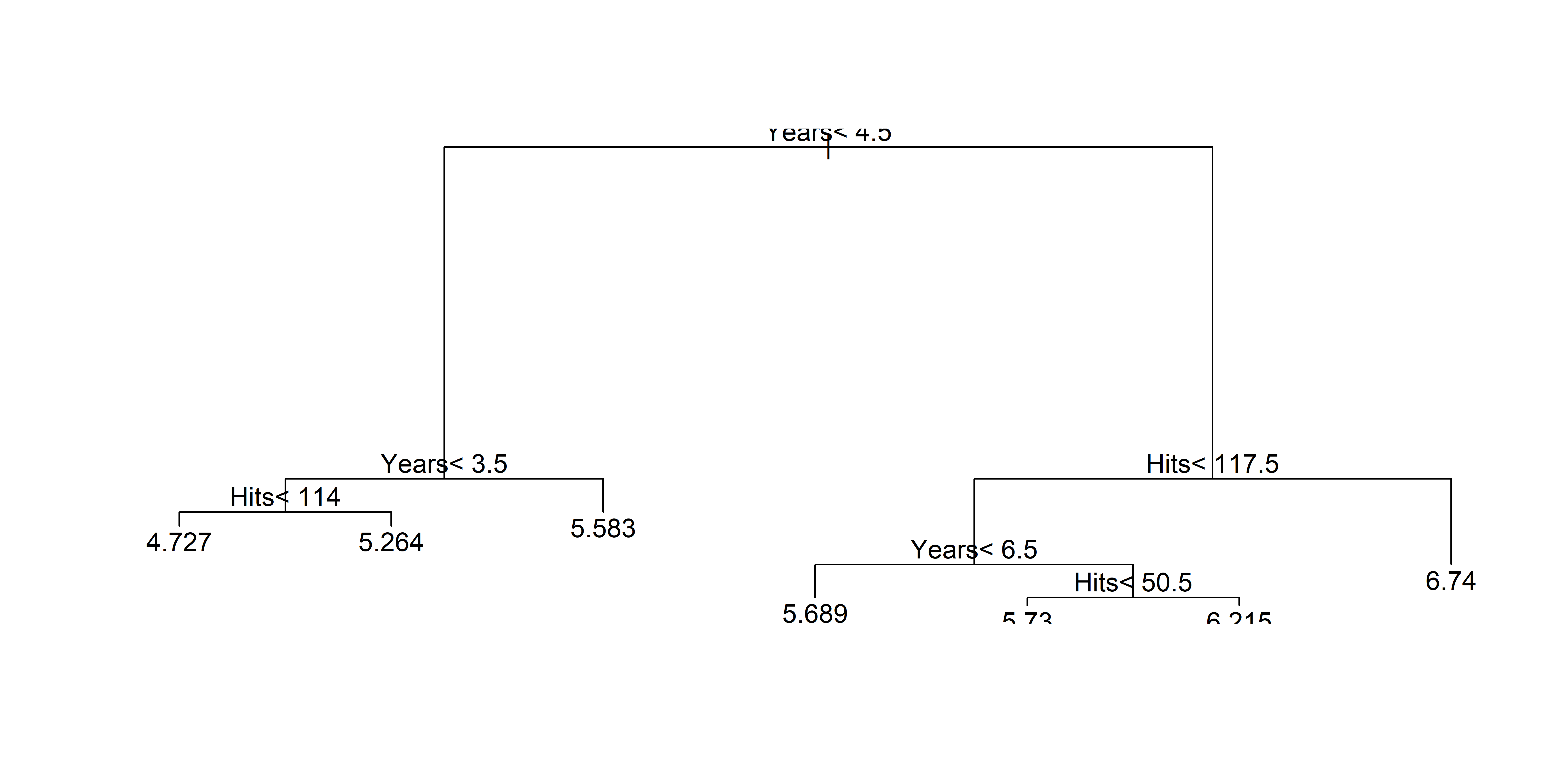
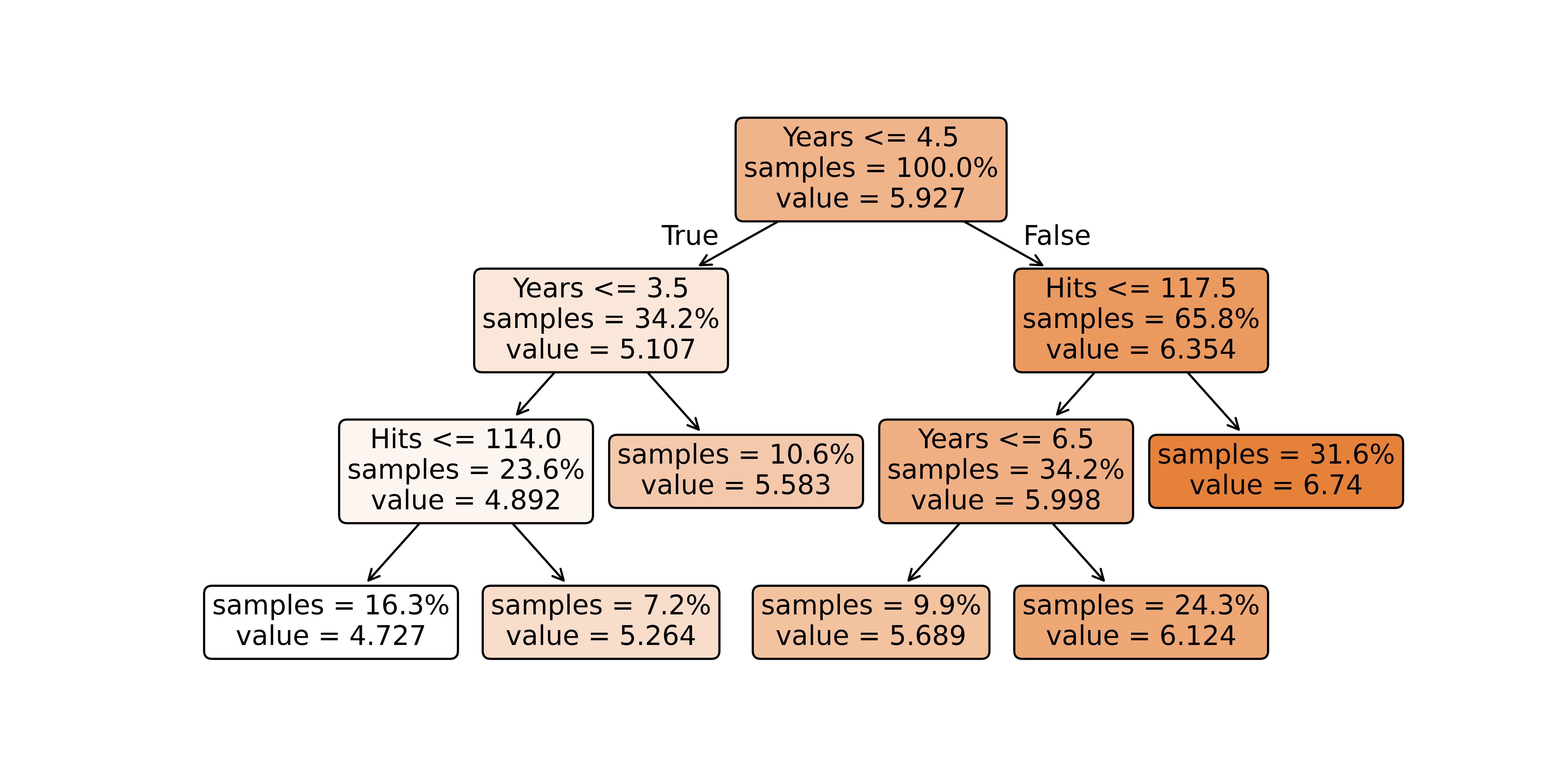
X = hitters[['Years', 'Hits']]
y = np.log(hitters['Salary'])
tree = DecisionTreeRegressor(min_samples_split=20, min_samples_leaf=10, max_depth=3, ccp_alpha=0.01)
tree.fit(X, y);
print(export_text(tree, feature_names=['Years', 'Hits']))
|--- Years <= 4.50
| |--- Years <= 3.50
| | |--- Hits <= 114.00
| | | |--- value: [4.73]
| | |--- Hits > 114.00
| | | |--- value: [5.26]
| |--- Years > 3.50
| | |--- value: [5.58]
|--- Years > 4.50
| |--- Hits <= 117.50
| | |--- Years <= 6.50
| | | |--- value: [5.69]
| | |--- Years > 6.50
| | | |--- value: [6.12]
| |--- Hits > 117.50
| | |--- value: [6.74]Nicer plots for decision trees
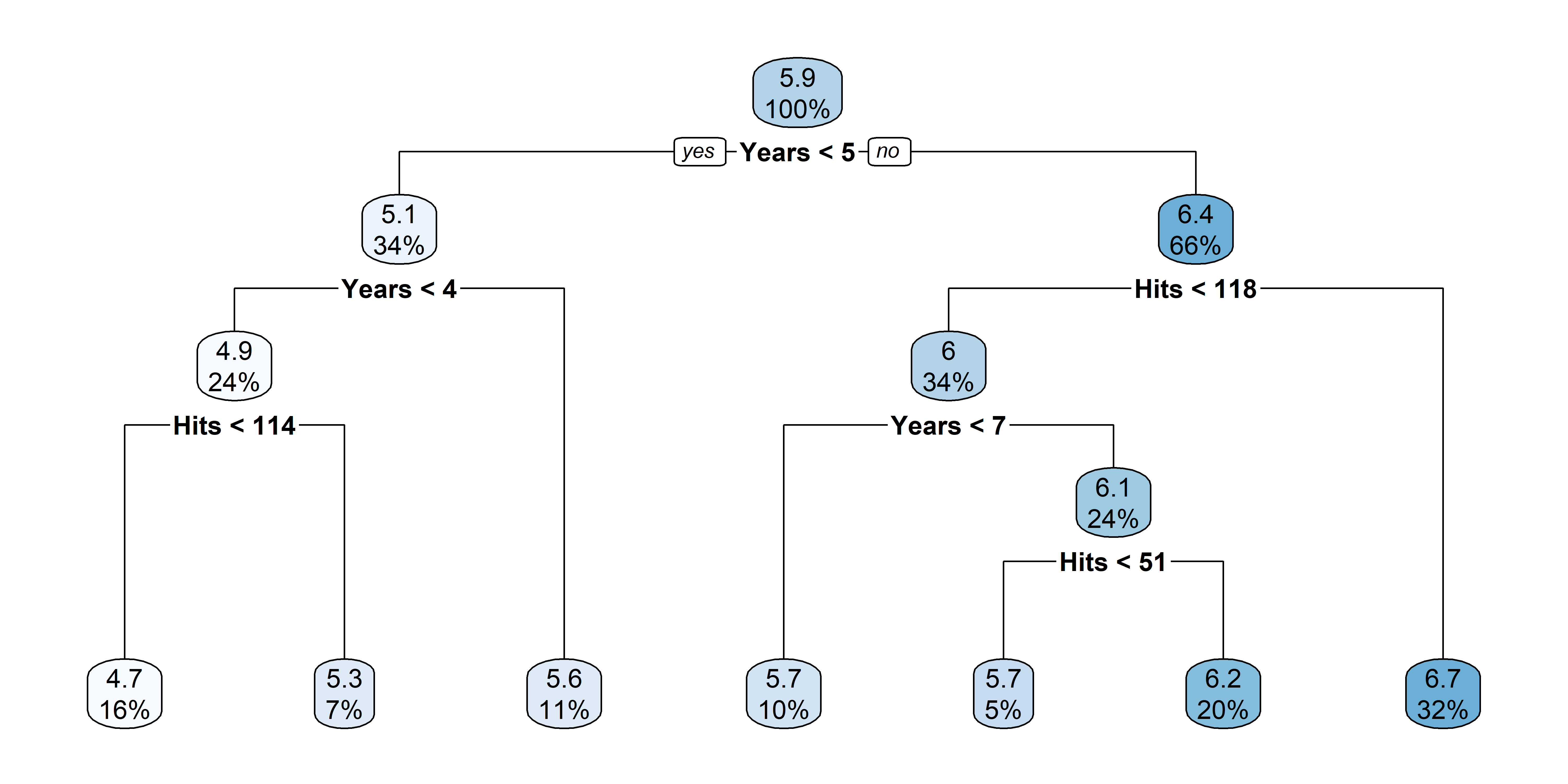
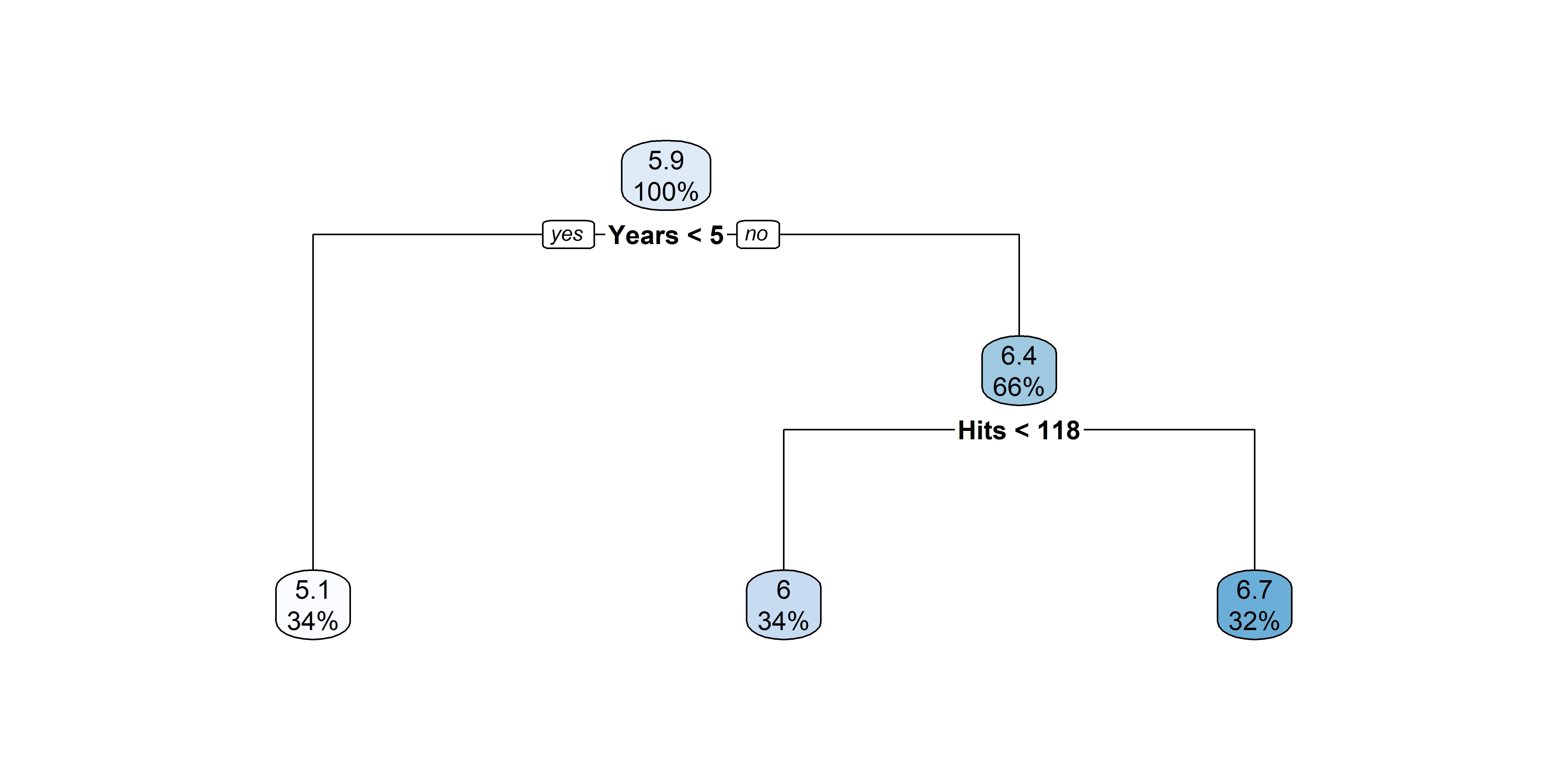
After pruning that tree

Tree Terminology
Regions in the predictor space
Code
ggplot(Hitters, aes(x = Years, y = Hits, colour = log(Salary))) +
  geom_point() +
  geom_vline(xintercept = 4.5, colour = "black", linetype = "dashed") +
  annotate("segment", x = 4.5, xend = 24, y = 117.5, yend = 117.5, colour = "black", linetype = "dashed") +
  annotate("text", x = 2, y = 200, label = "R[1]", parse = TRUE, size = 10) +
  annotate("text", x = 20, y = 50, label = "R[2]", parse = TRUE, size = 10) +
  annotate("text", x = 20, y = 200, label = "R[3]", parse = TRUE, size = 10) +
  theme(text = element_text(size = 20))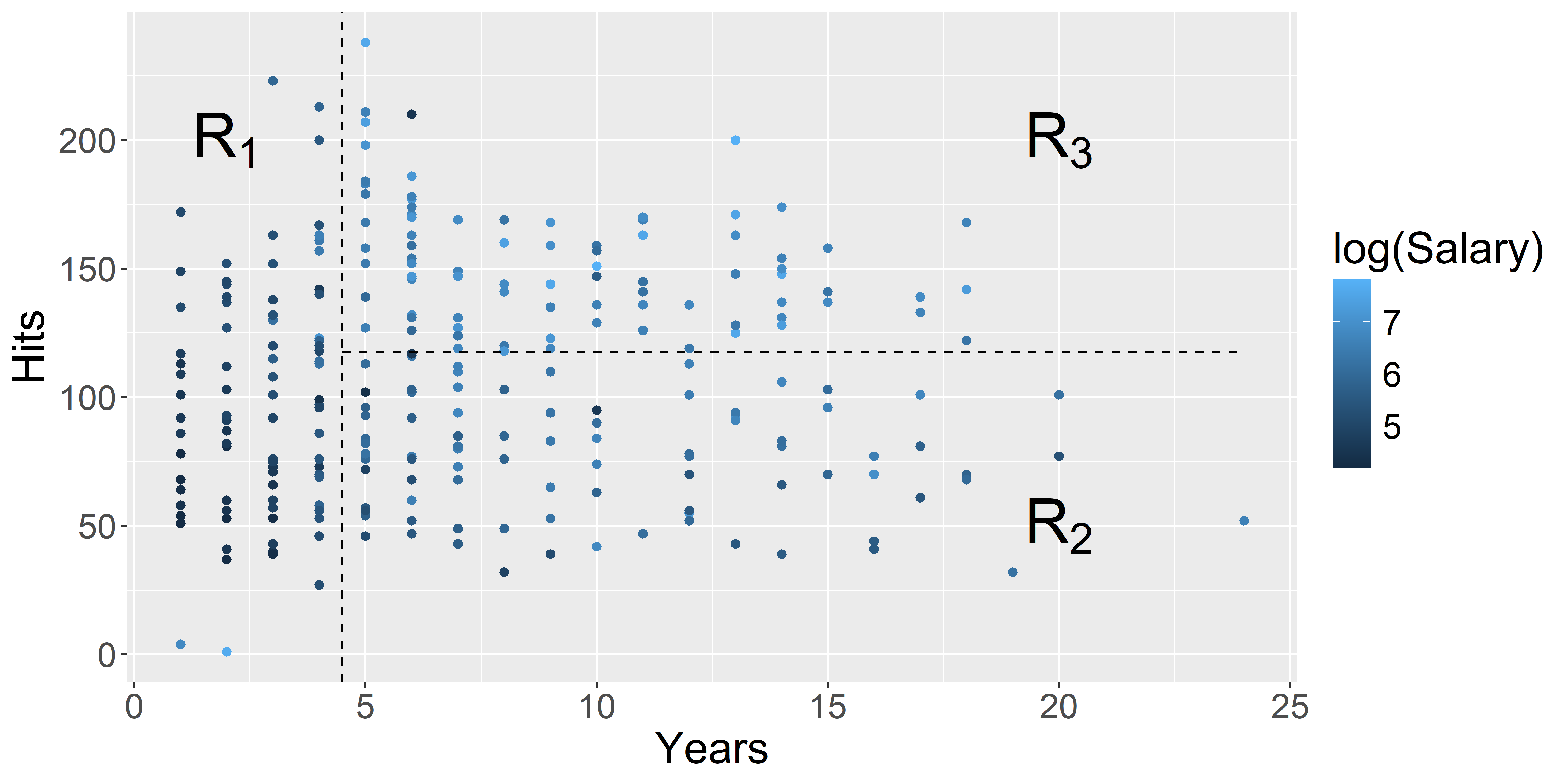
Discussion

Decision trees: summary
- Decision trees are simple, popular, and easy to interpret.
- They are not the most accurate method, but they can be great to understand the data.
- They do form the basis for more accurate and complex methods like random forests and boosting.
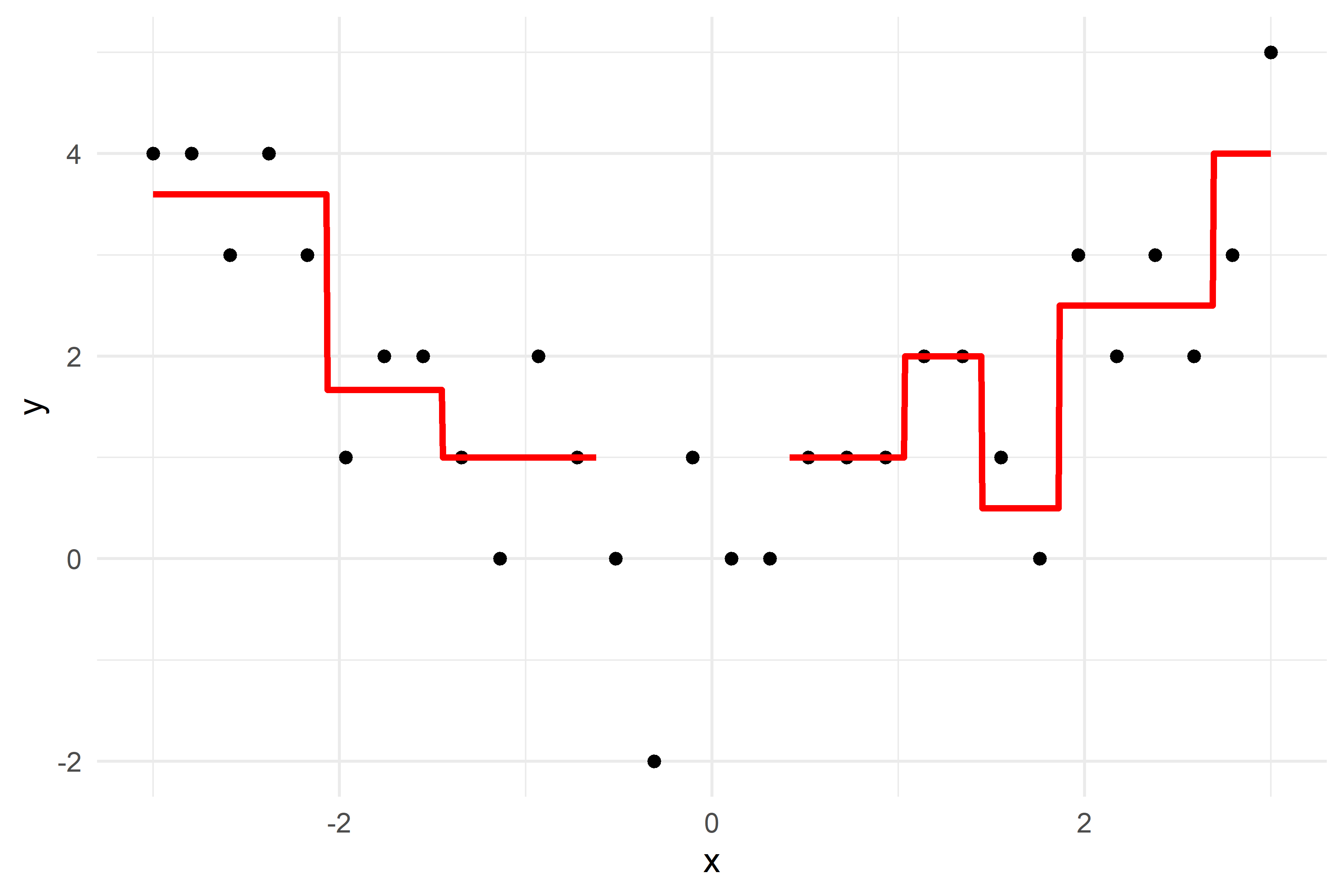
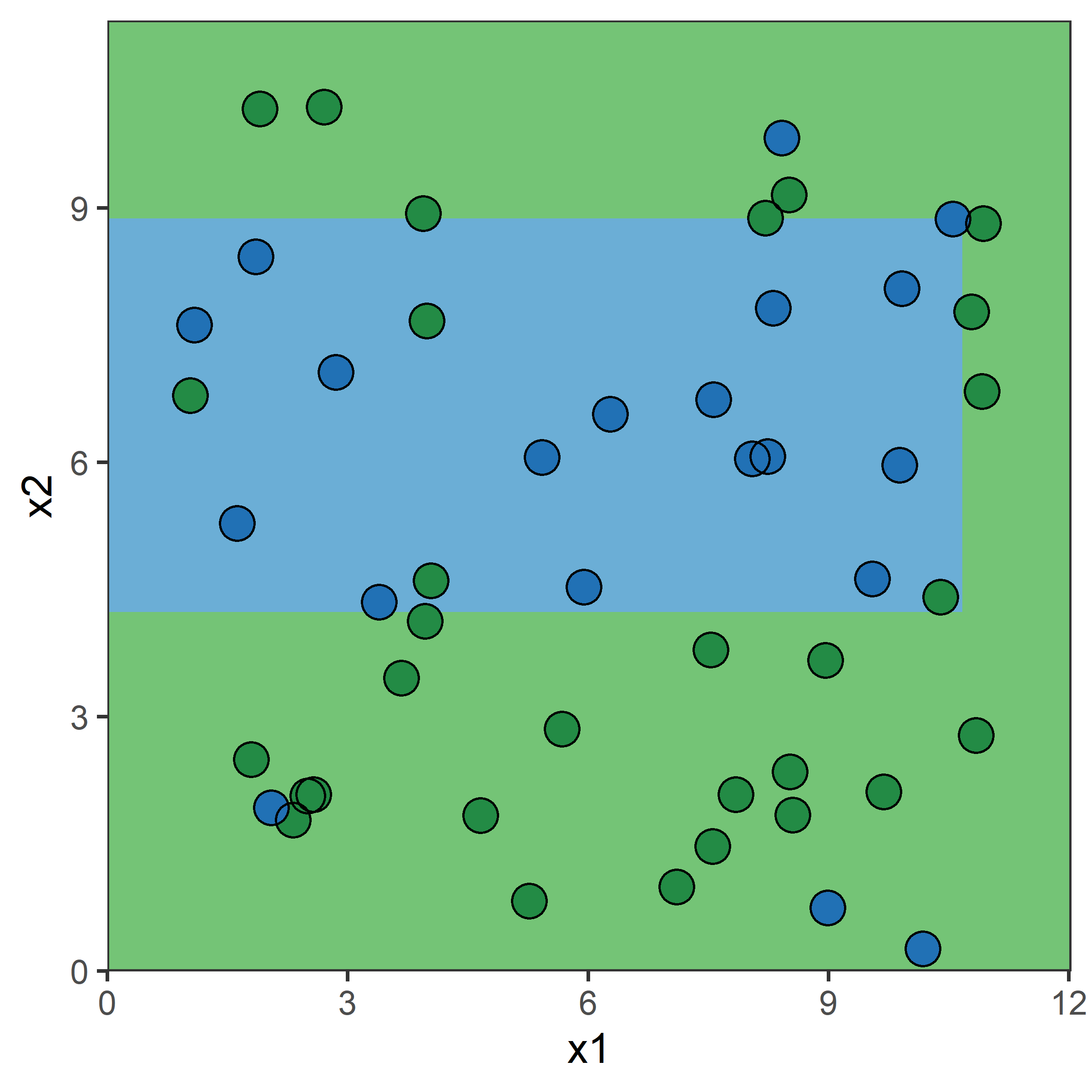
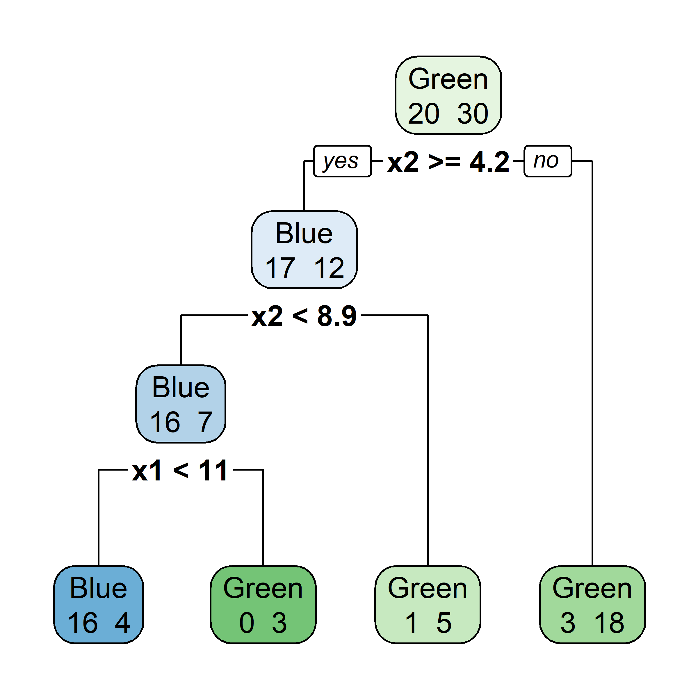
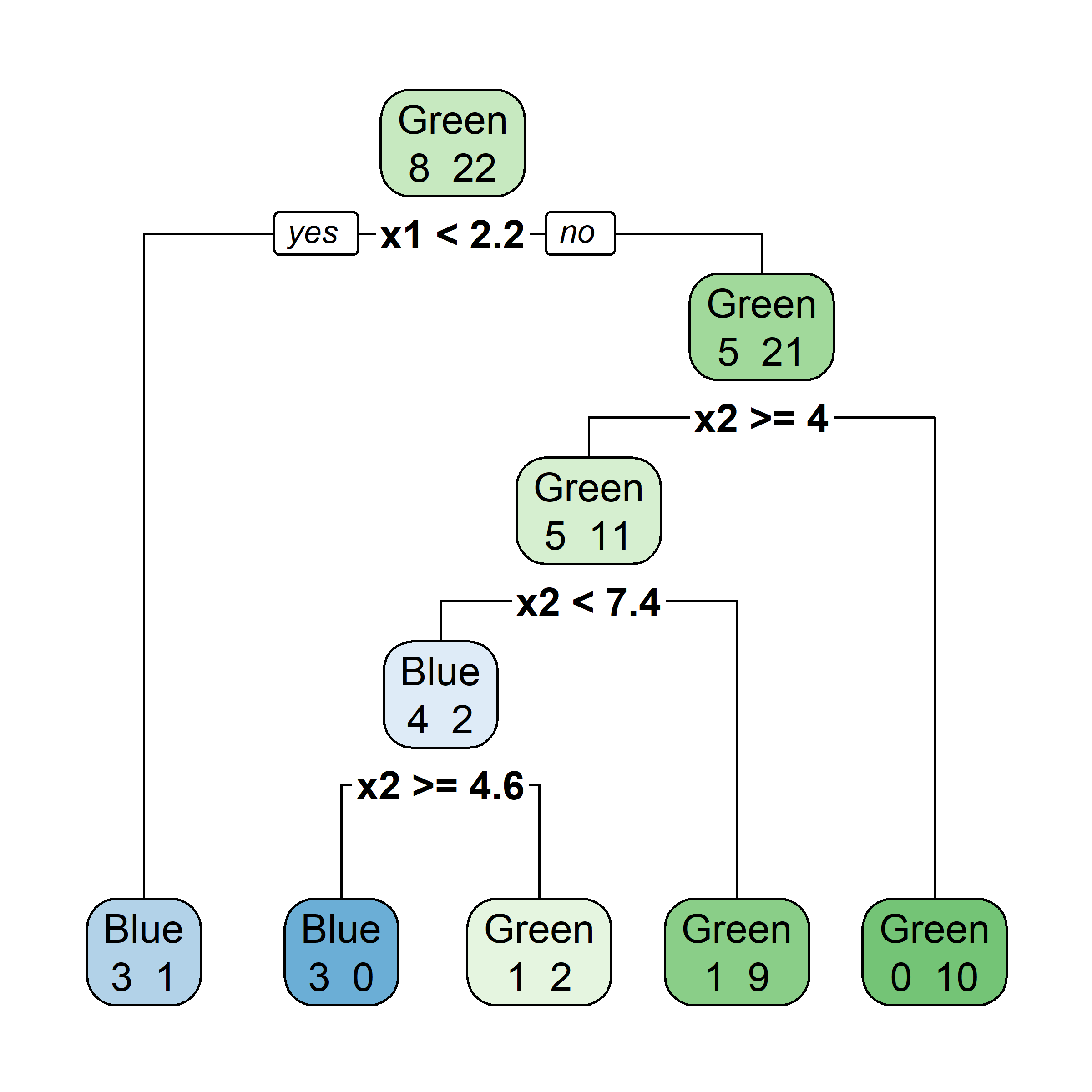
Illustraion with a synthetic regression dataset
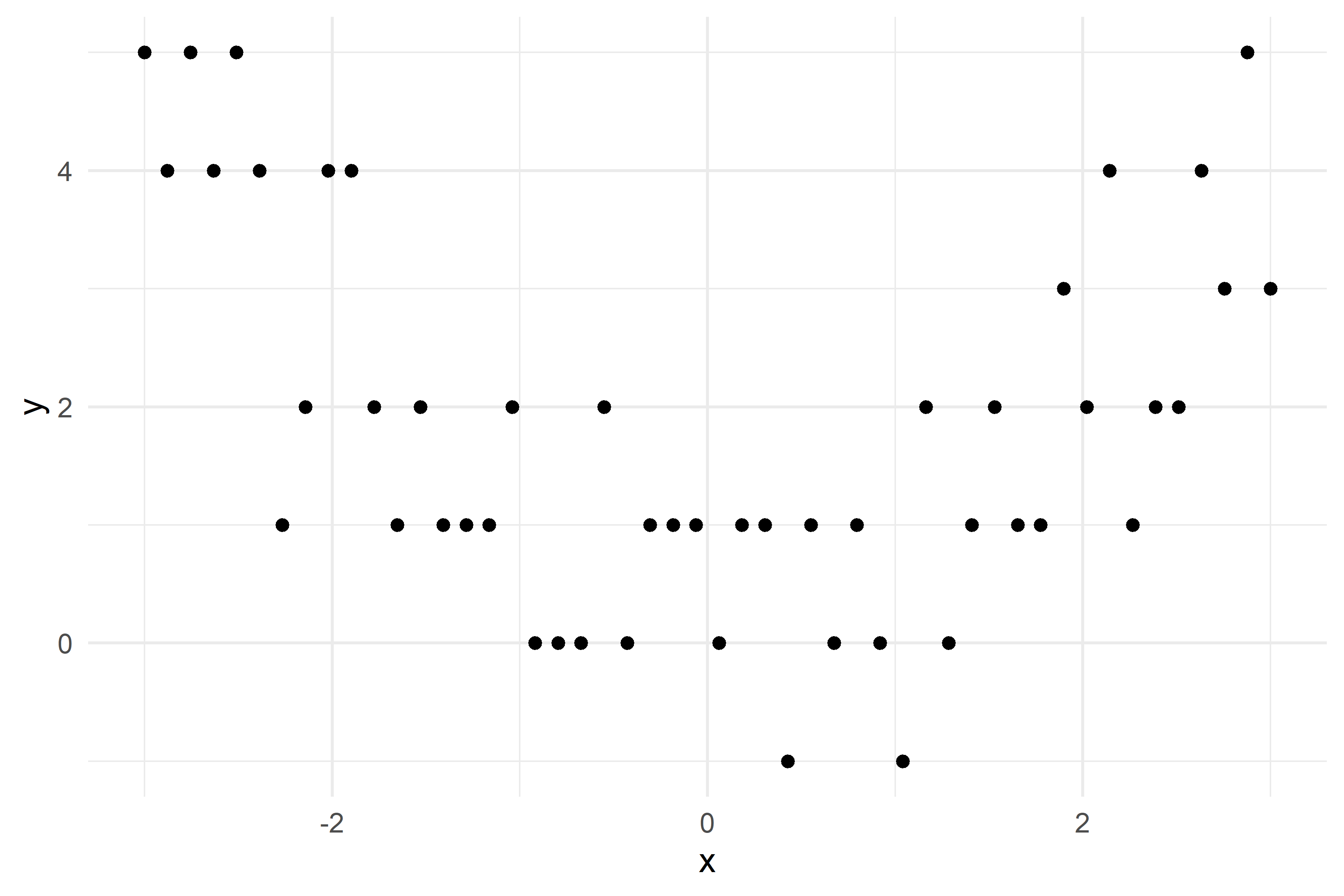
Growing a regression tree I
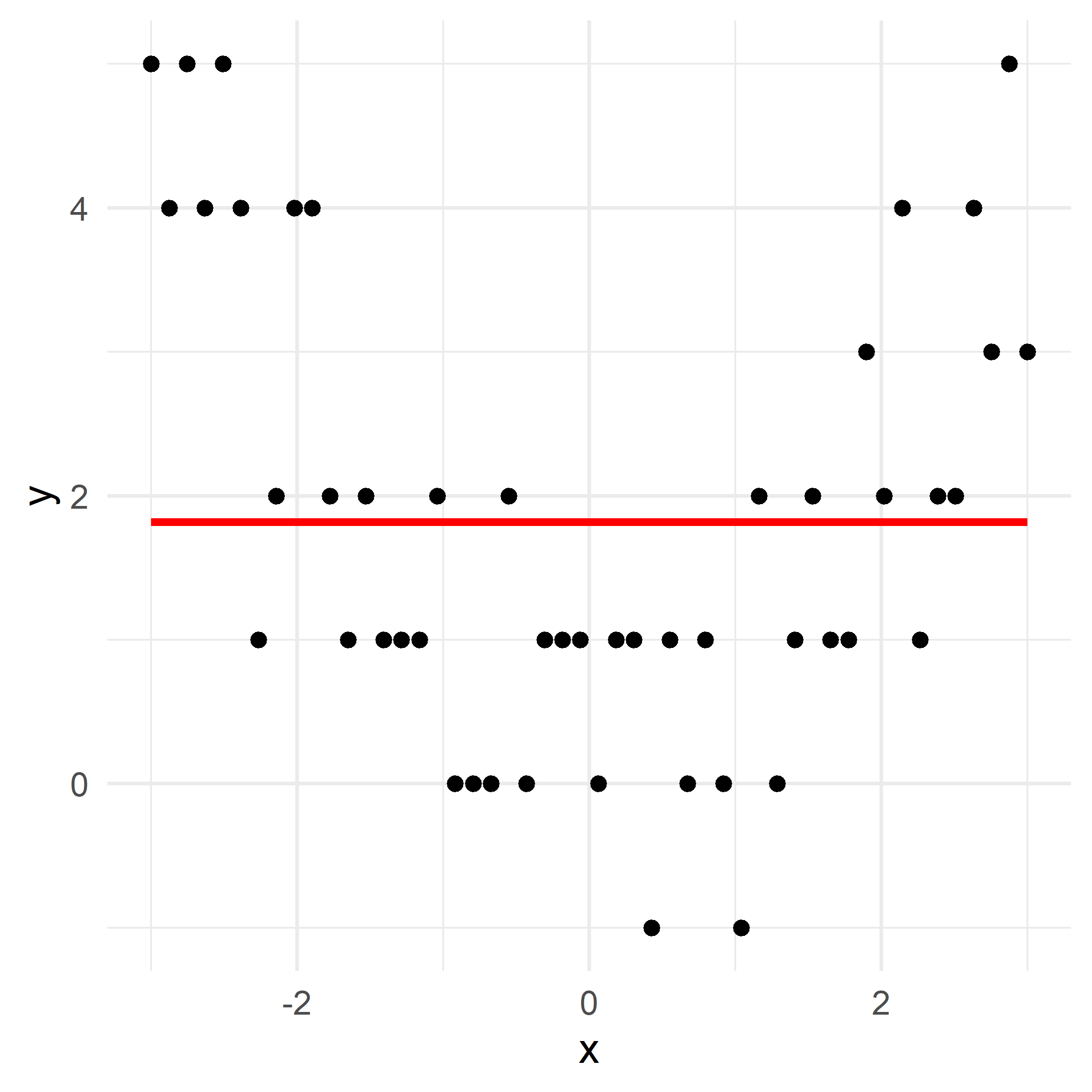

Growing a regression tree II
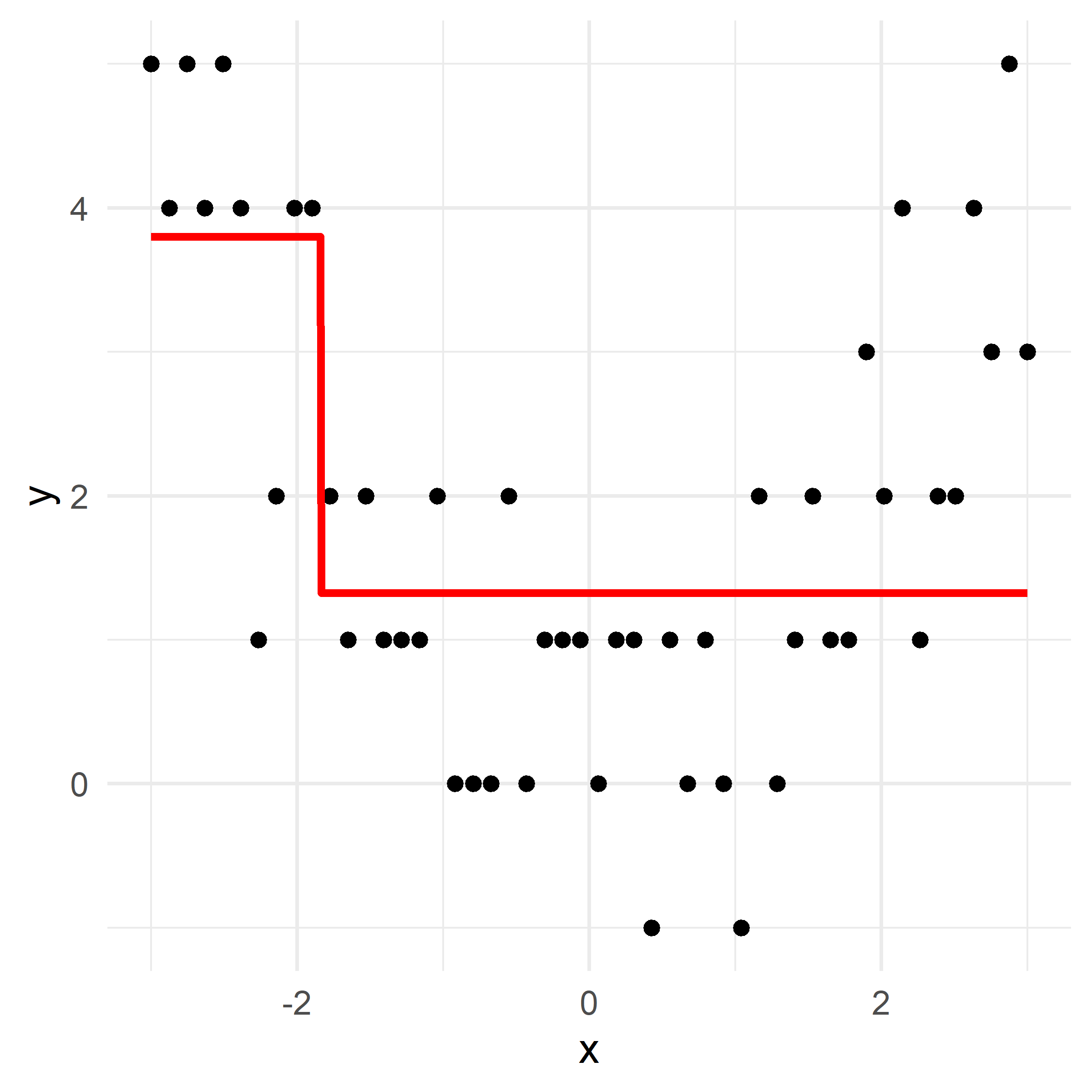
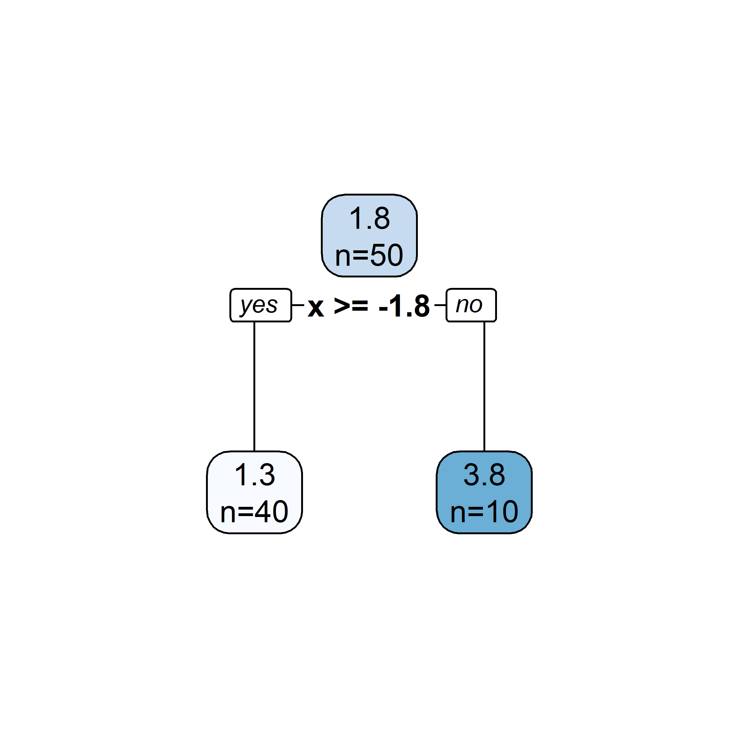
Growing a regression tree III
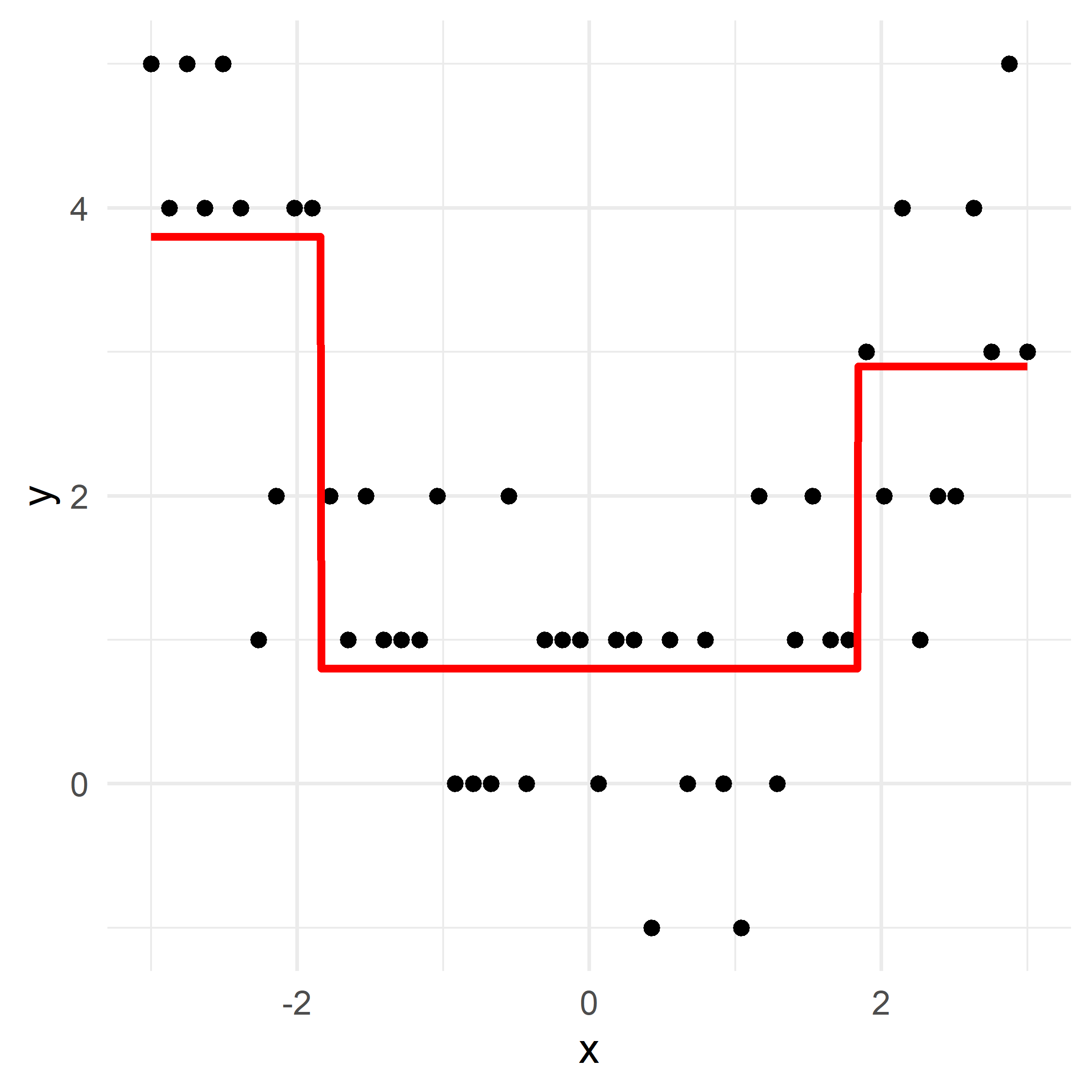
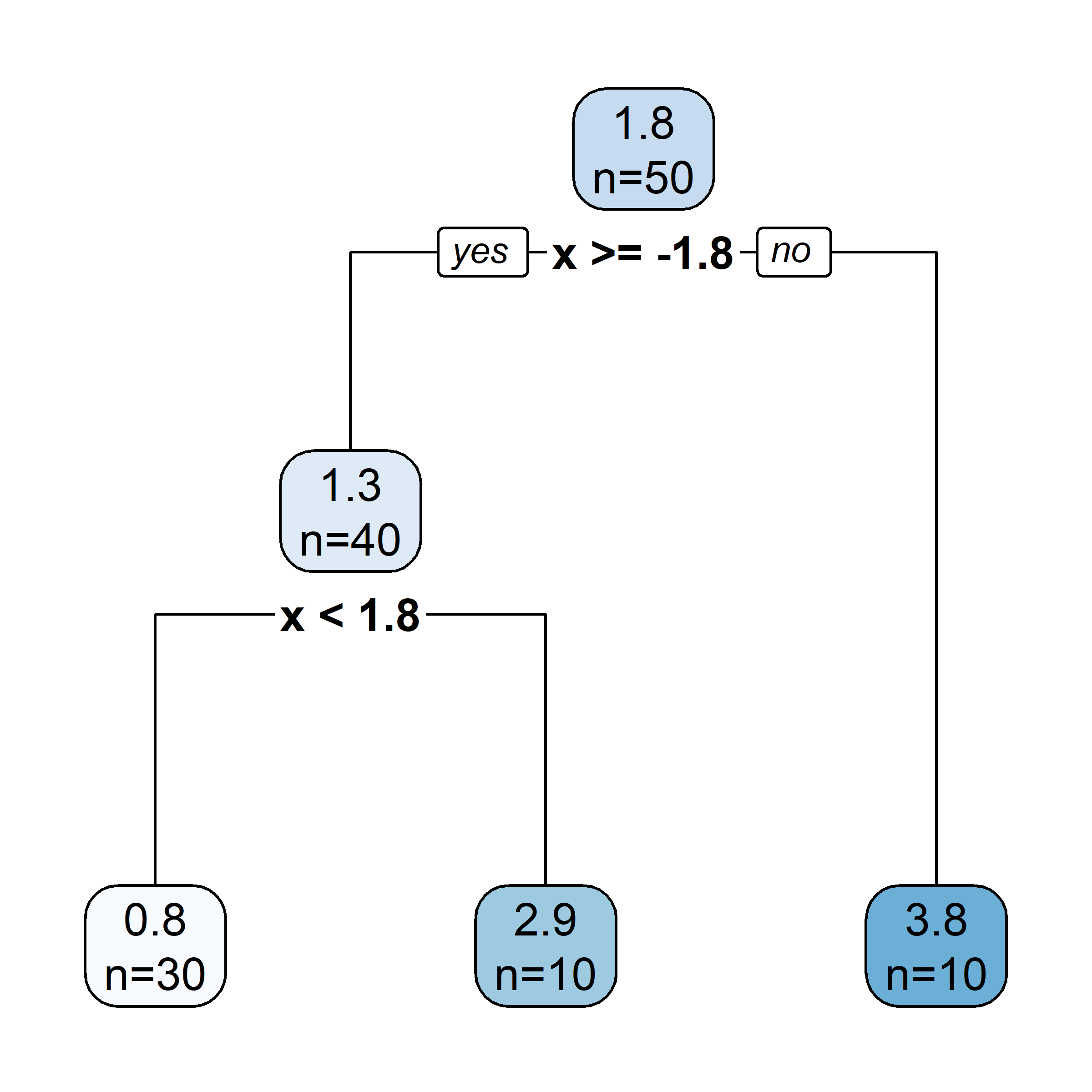
Growing a regression tree IV
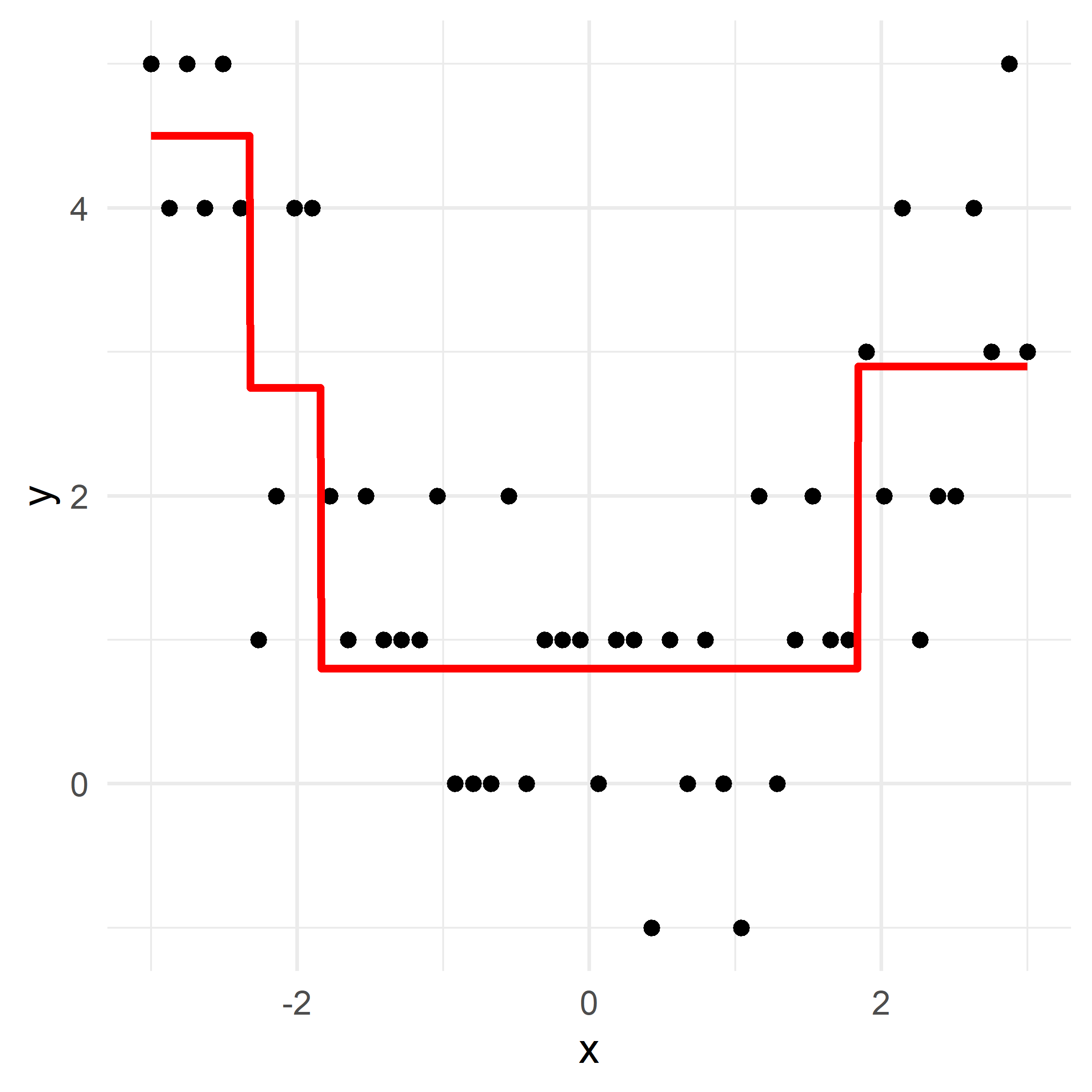
2023 exam question
What would be the tree’s predicted value for y at x = 0?
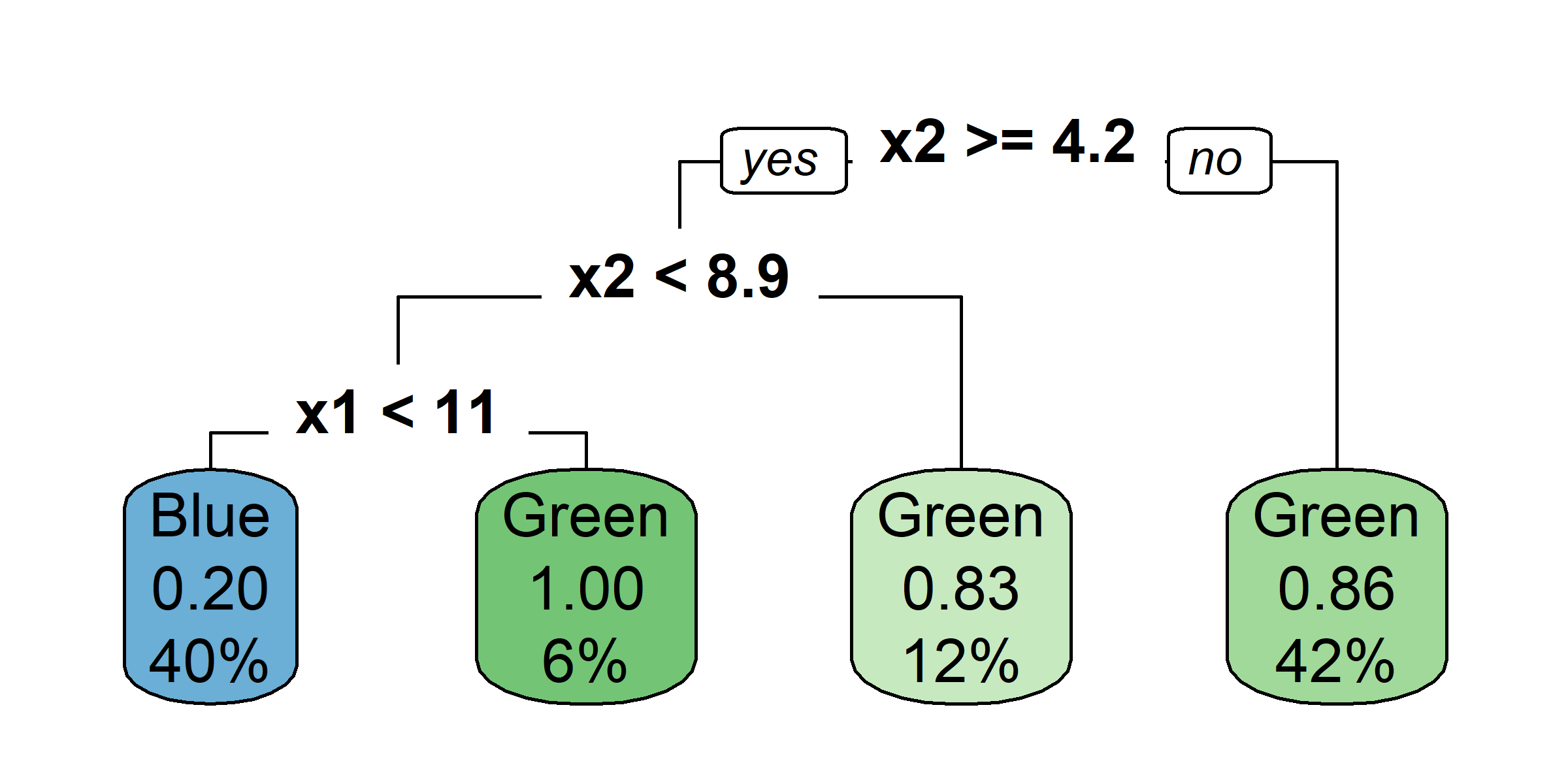
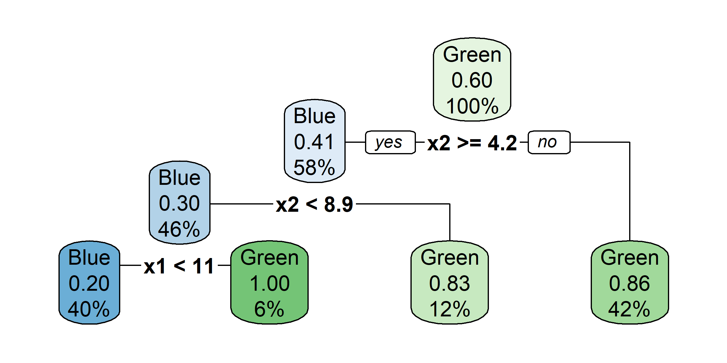
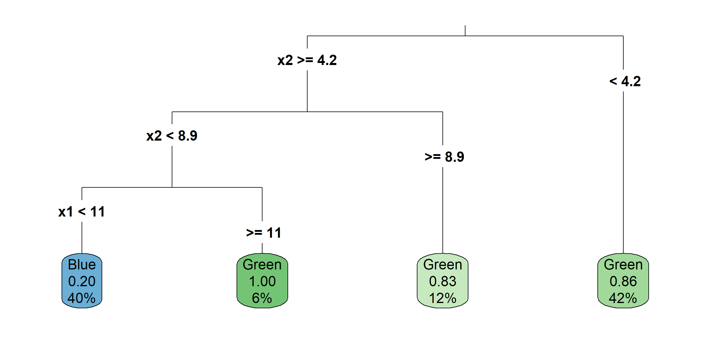
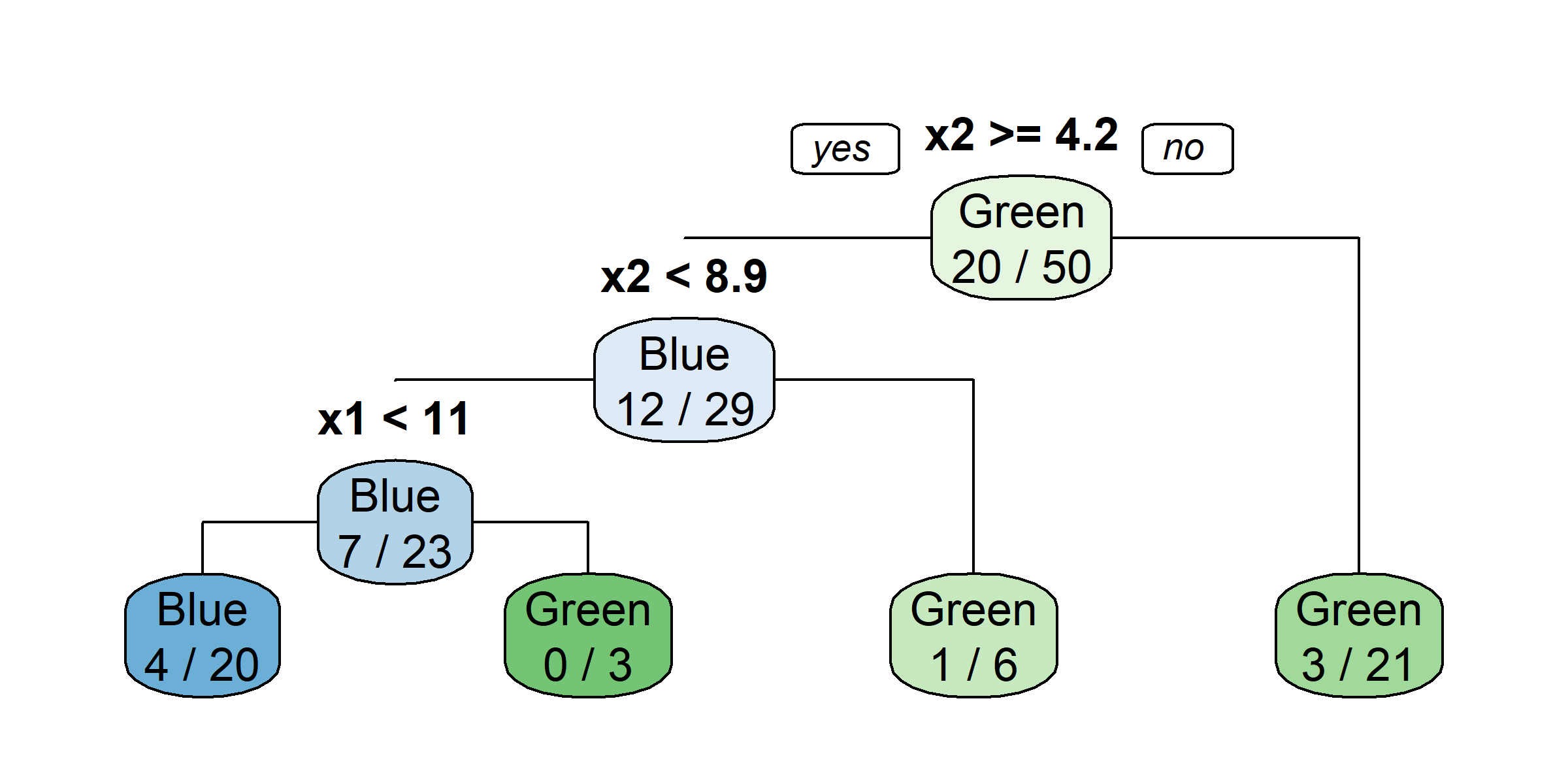
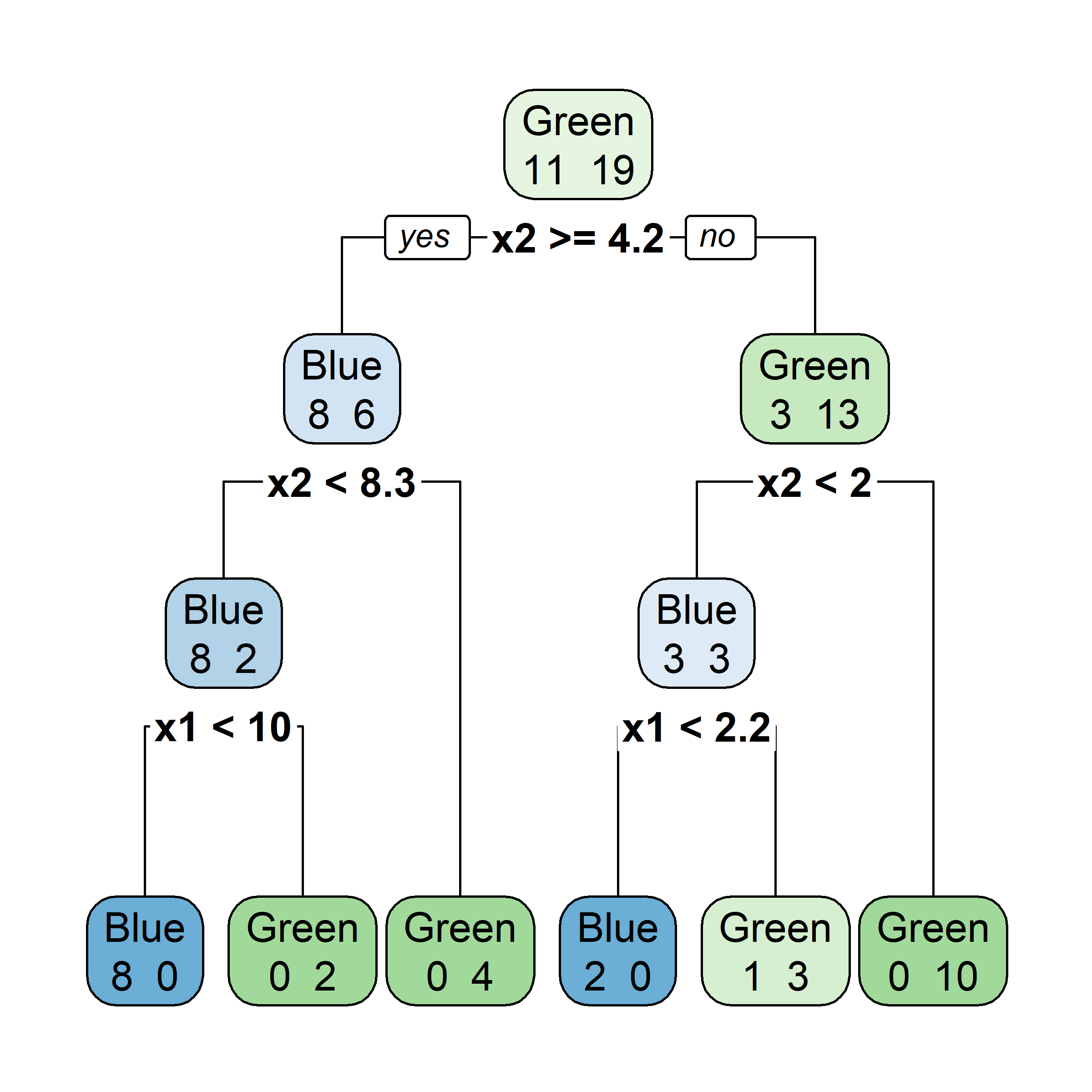
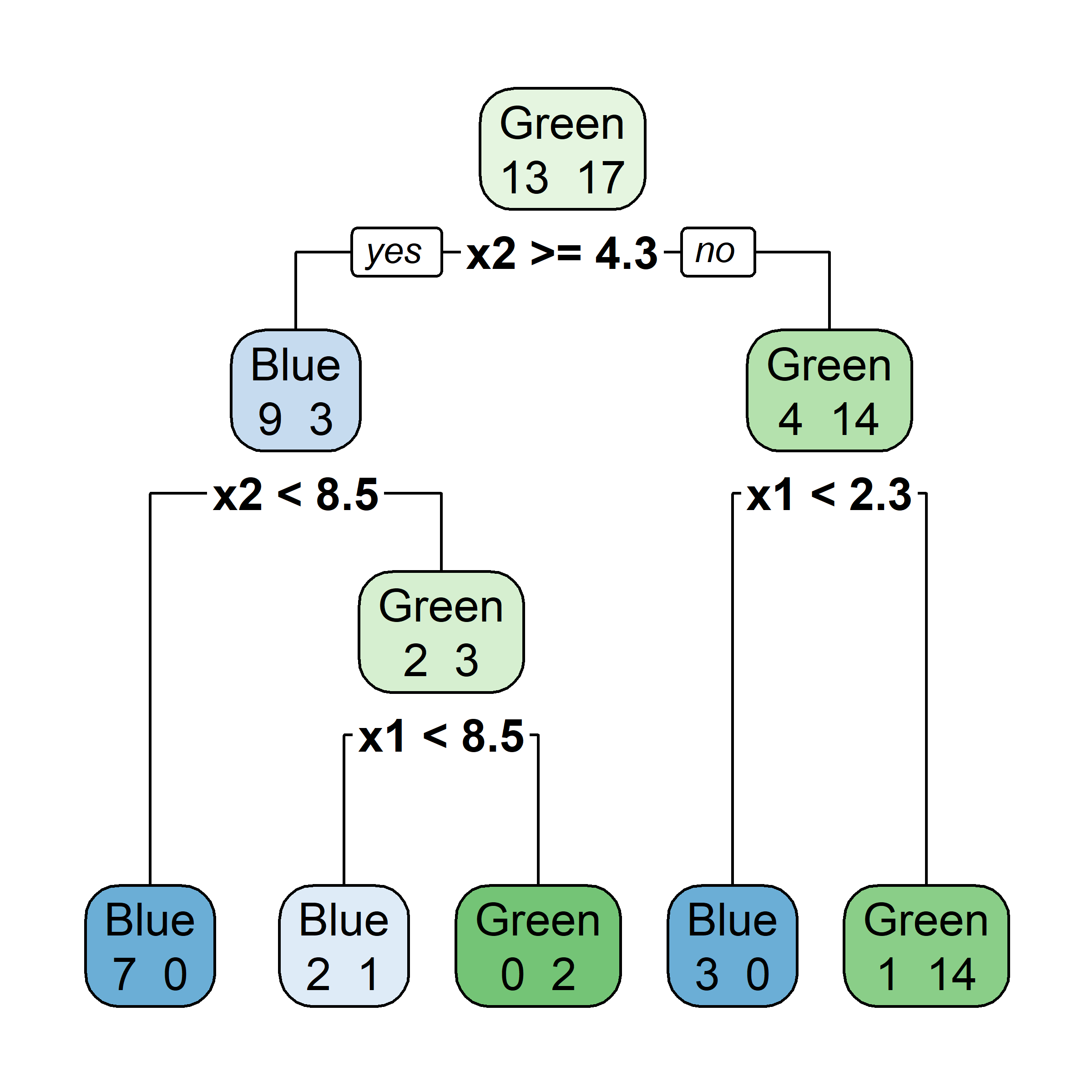
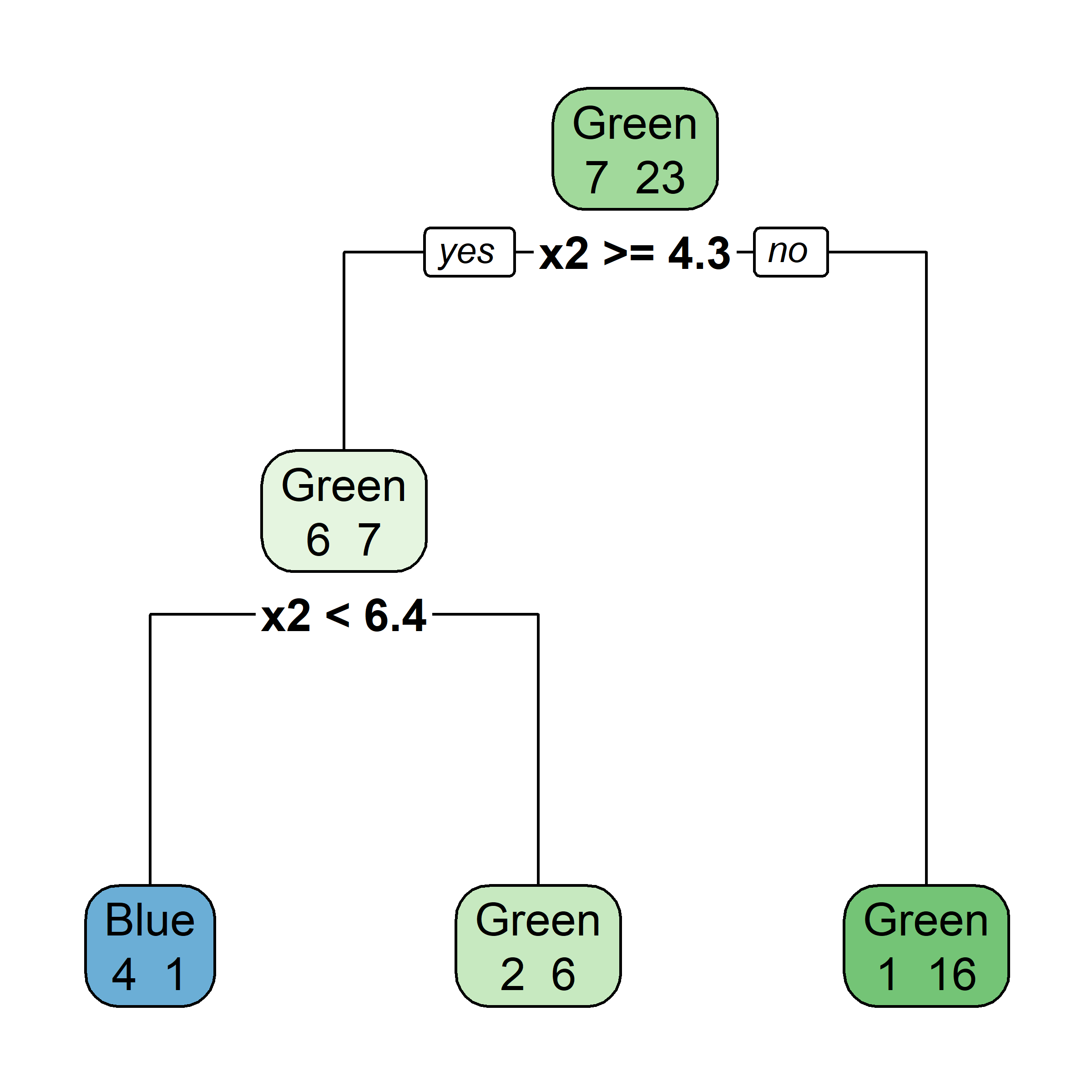
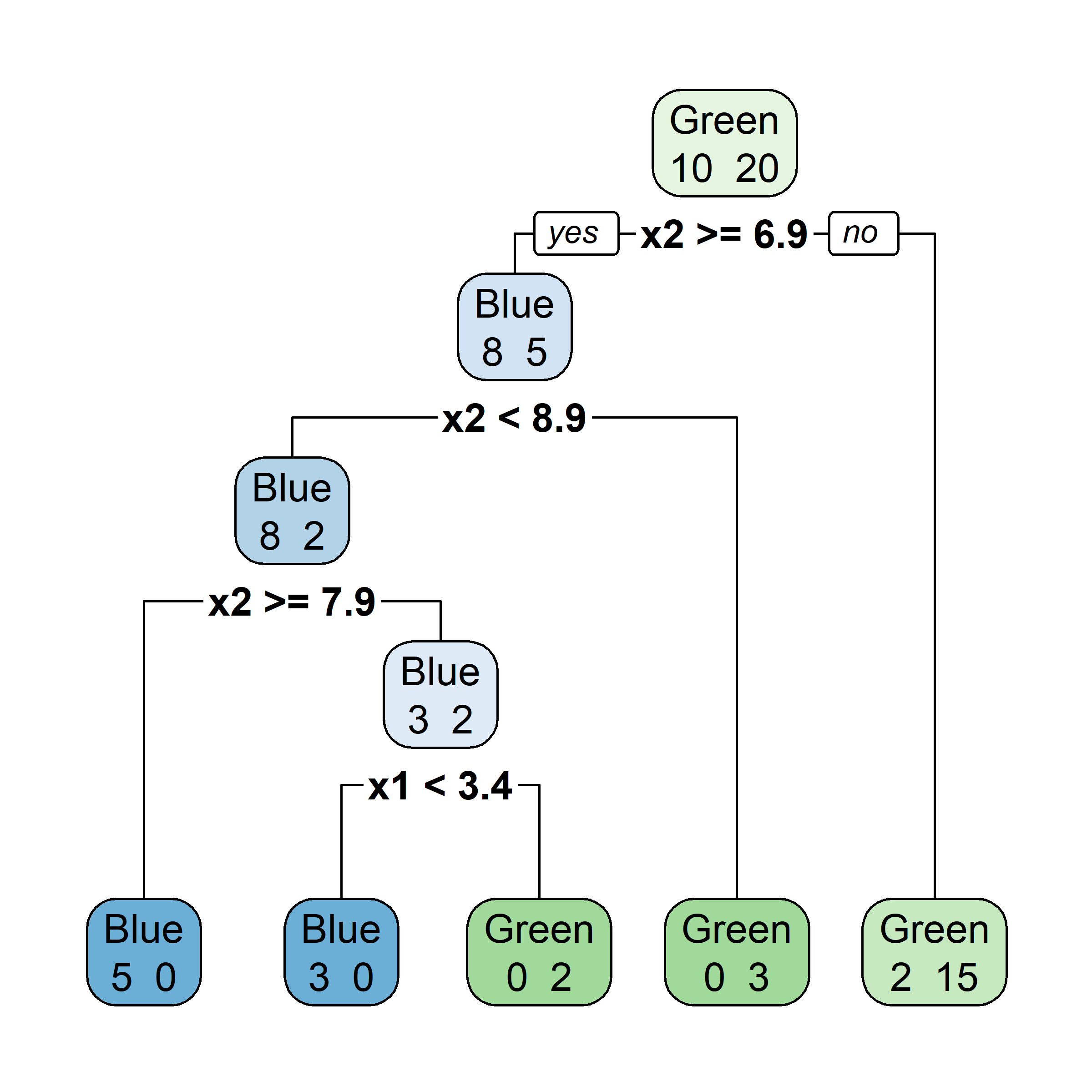
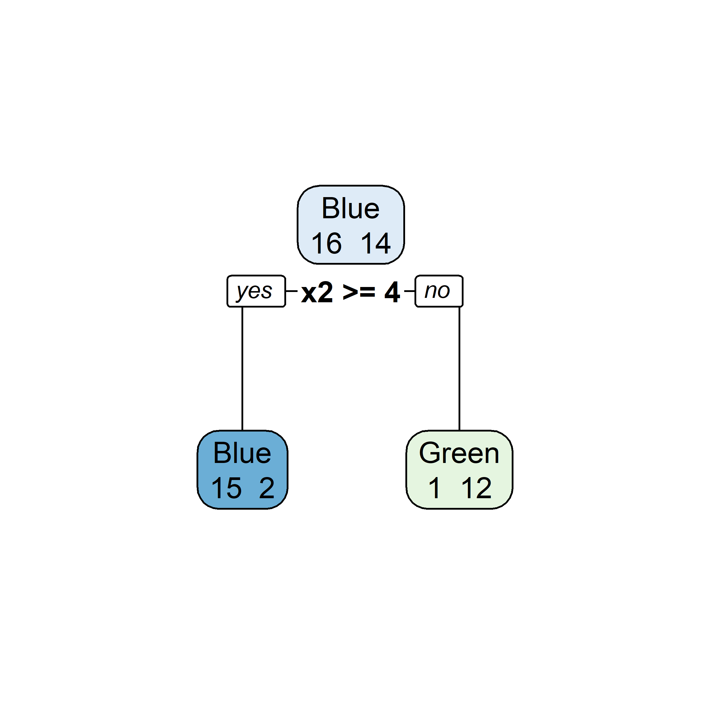
Growing a classification tree I
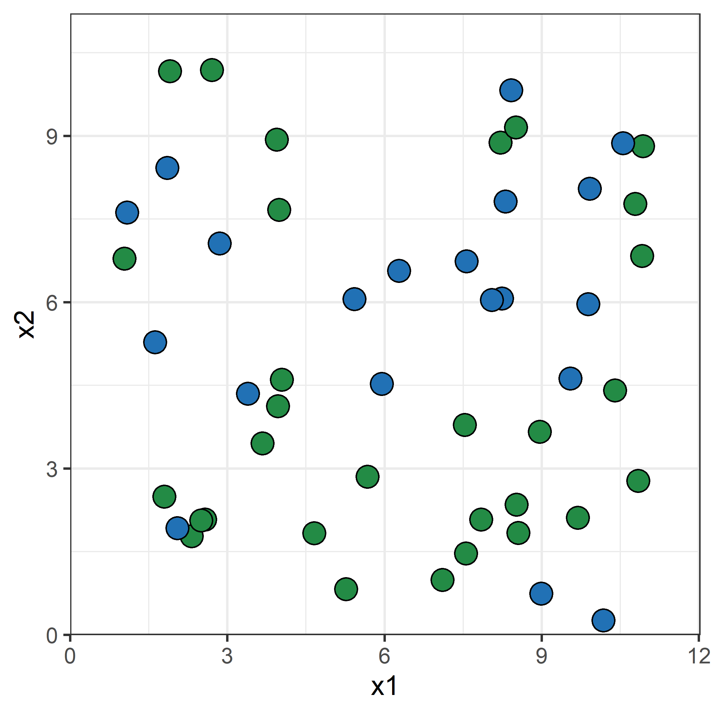

Growing a classification tree II
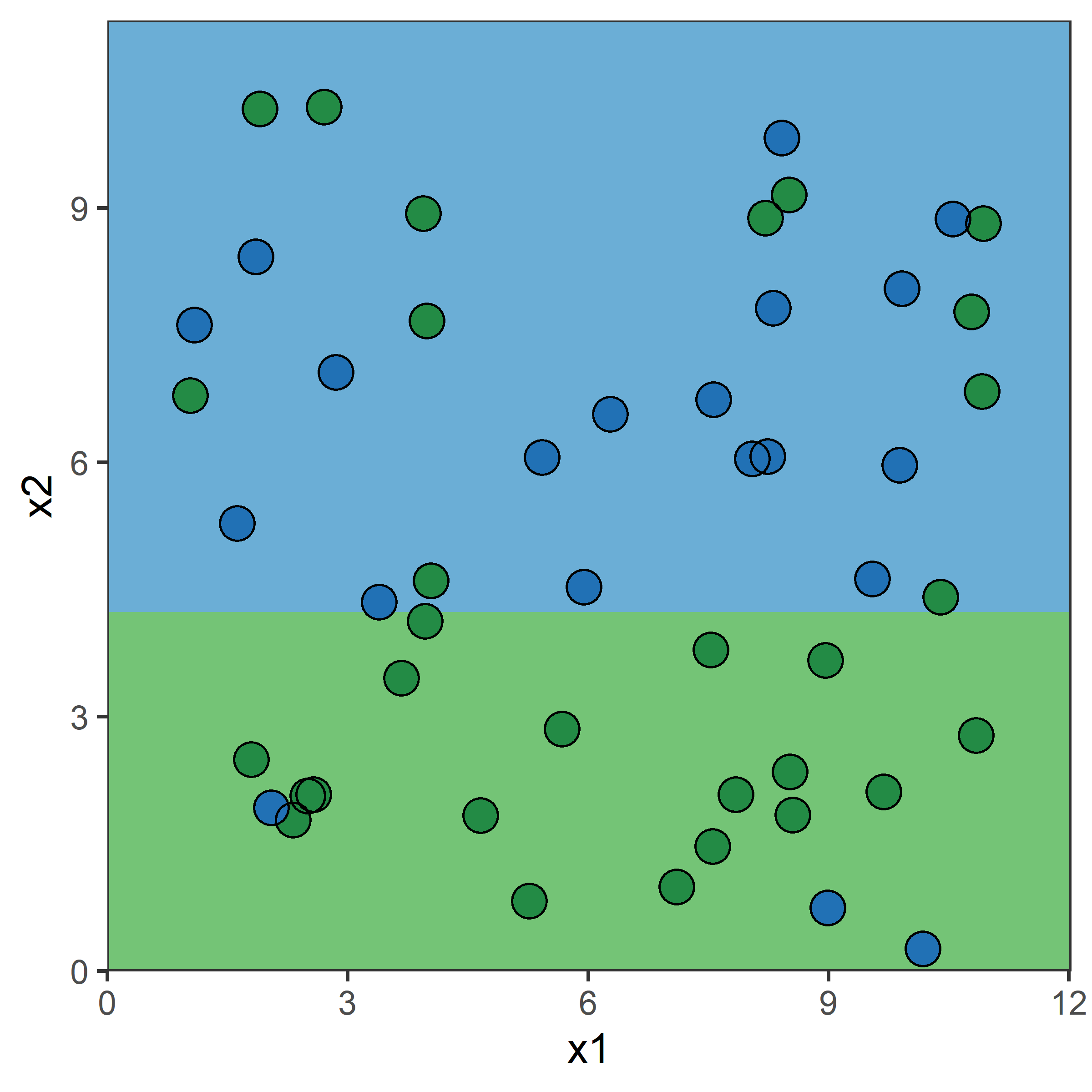
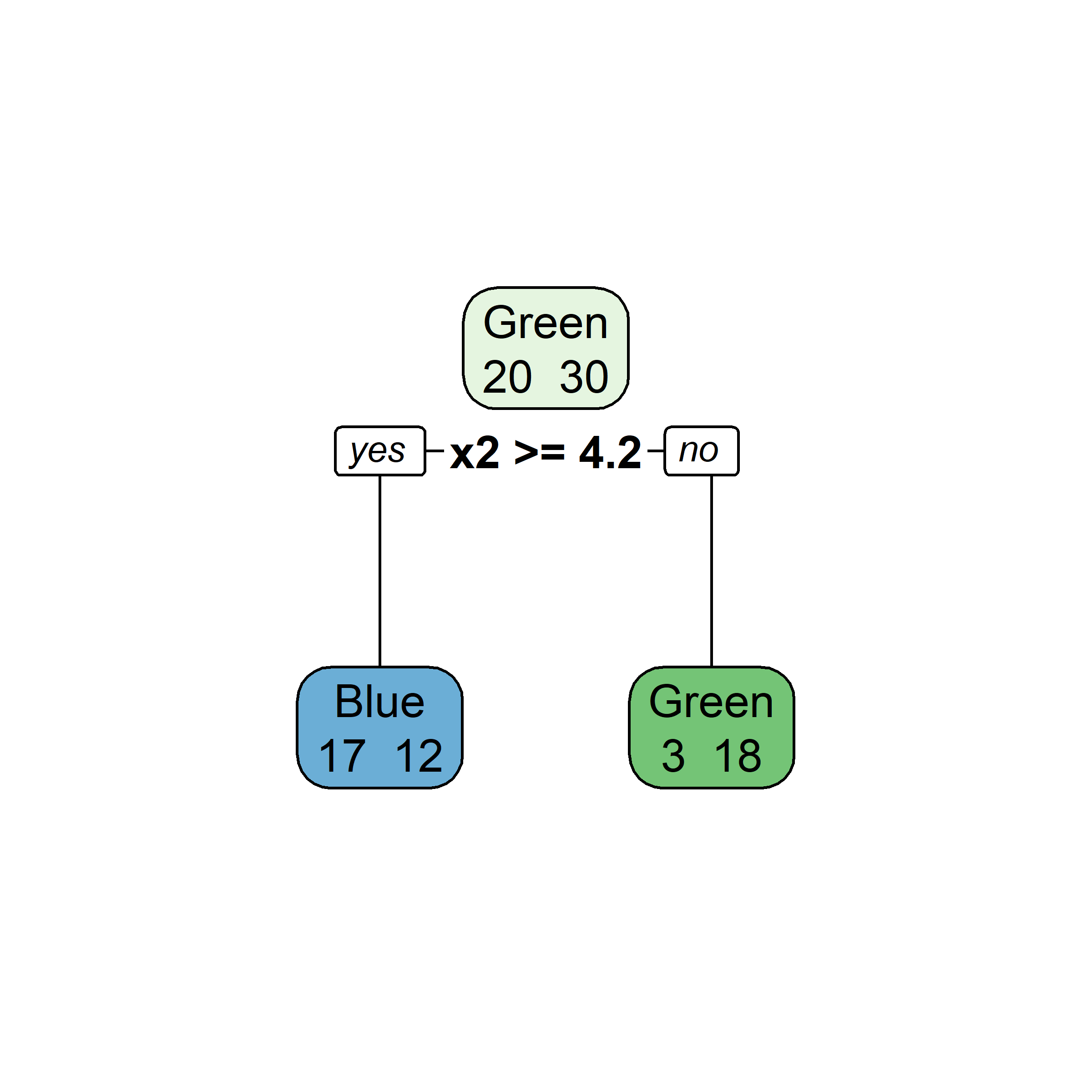
Growing a classification tree III
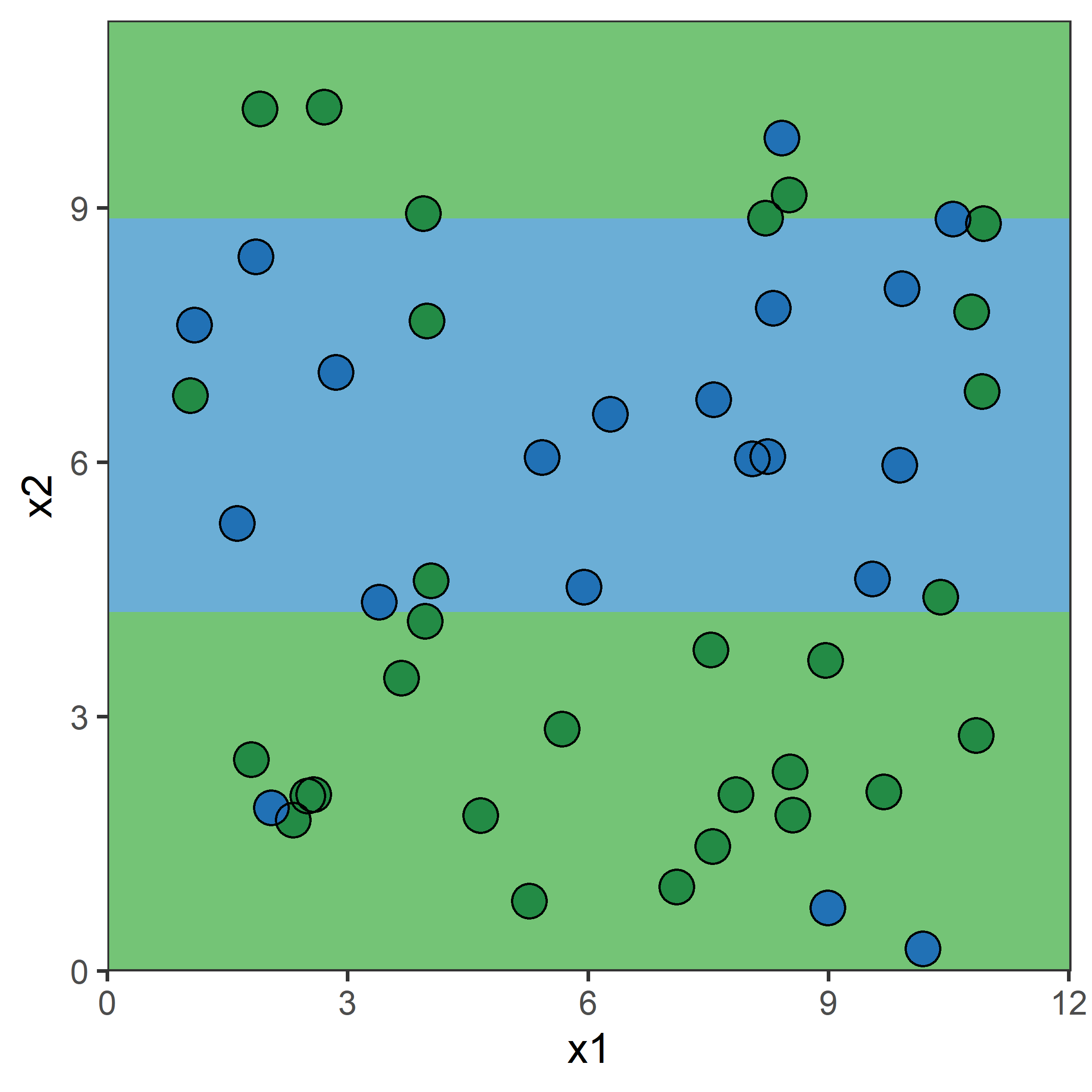
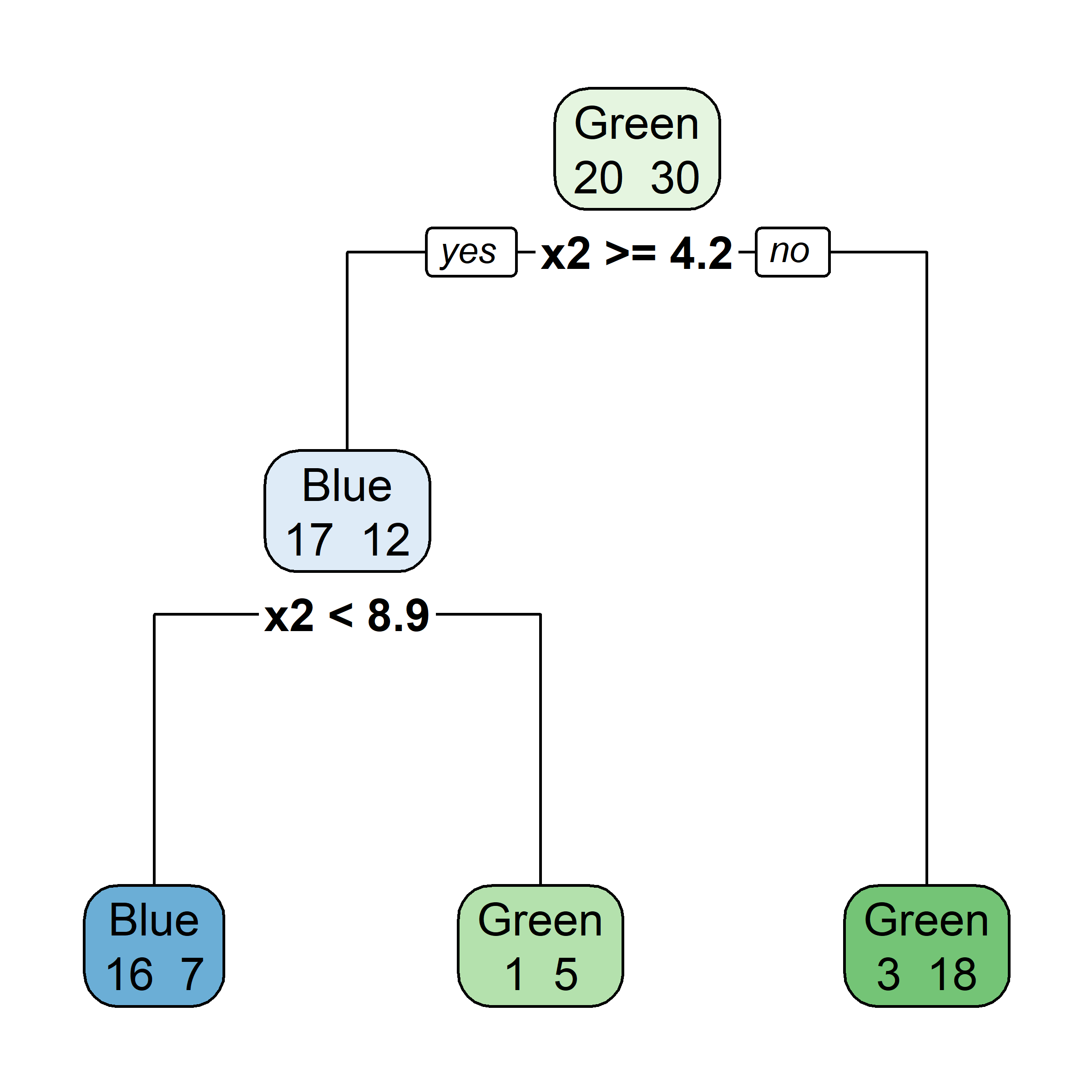
Growing a classification tree IV
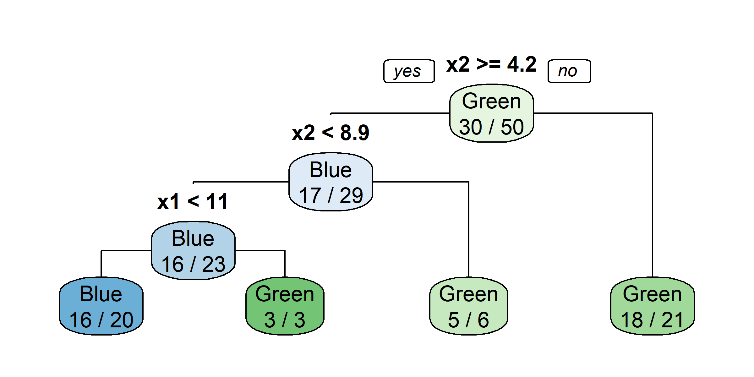
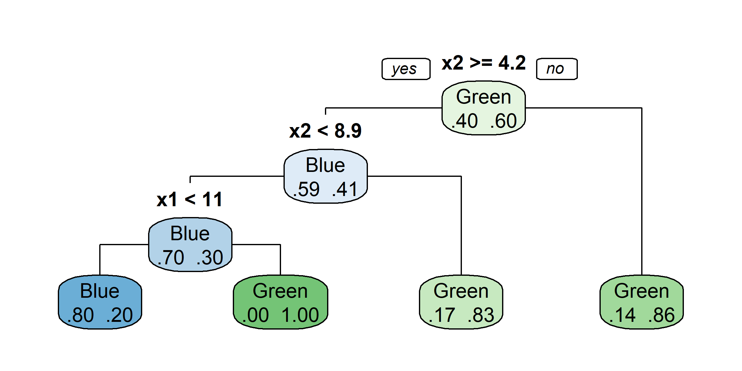
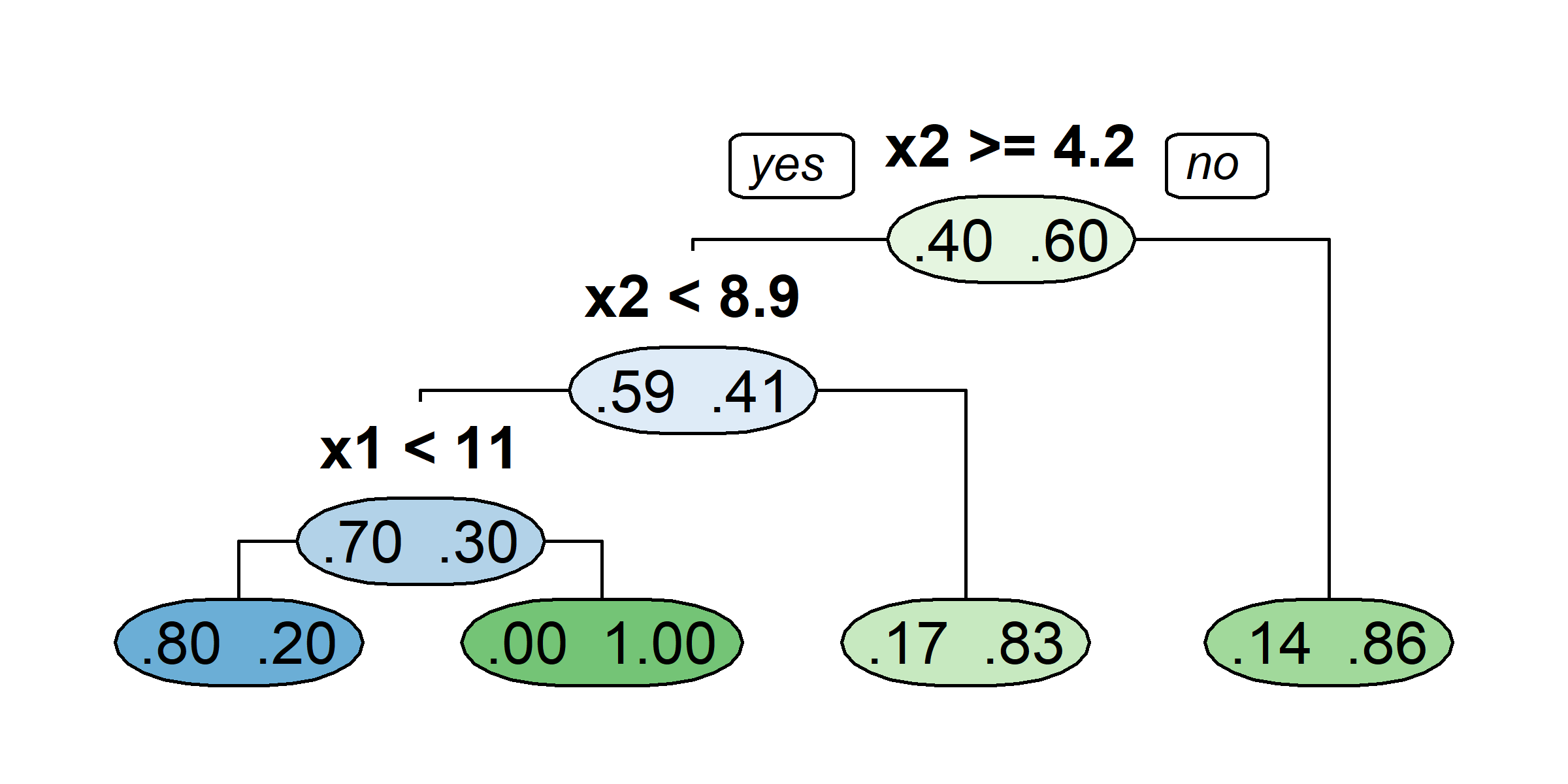
Multiple representations
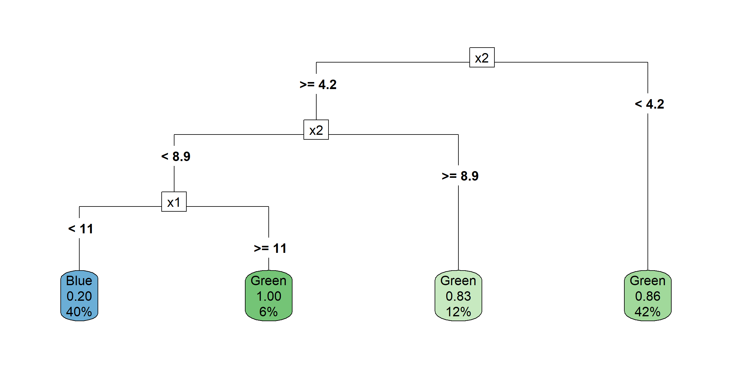
Multiple representations II
National Flood Insurance Program
Available at OpenFEMA dataset.

National Flood Insurance Program (NFIP, image source)
First decision tree

Remove ID column
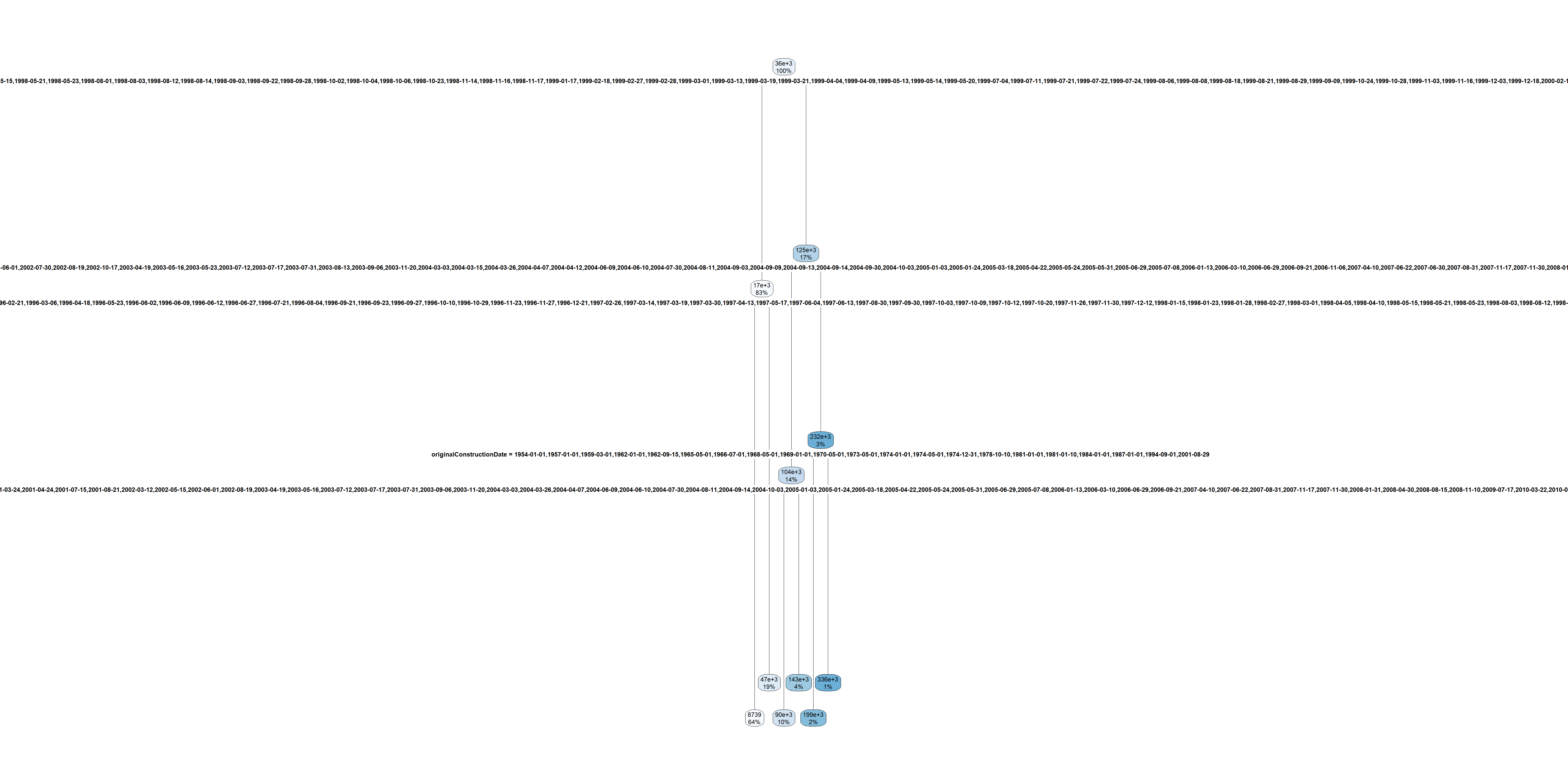
Dates to years and months
Code
claims$lossYear <- year(claims$lossDate)
claims$lossMonth <- month(claims$lossDate)
claims$lossDate <- NULL
claims$originalConstructionYear <- year(claims$originalConstructionDate)
claims$originalConstructionMonth <- month(claims$originalConstructionDate)
claims$originalConstructionDate <- NULL
claims$originalNBYear <- year(claims$originalNBDate)
claims$originalNBMonth <- month(claims$originalNBDate)
claims$originalNBDate <- NULL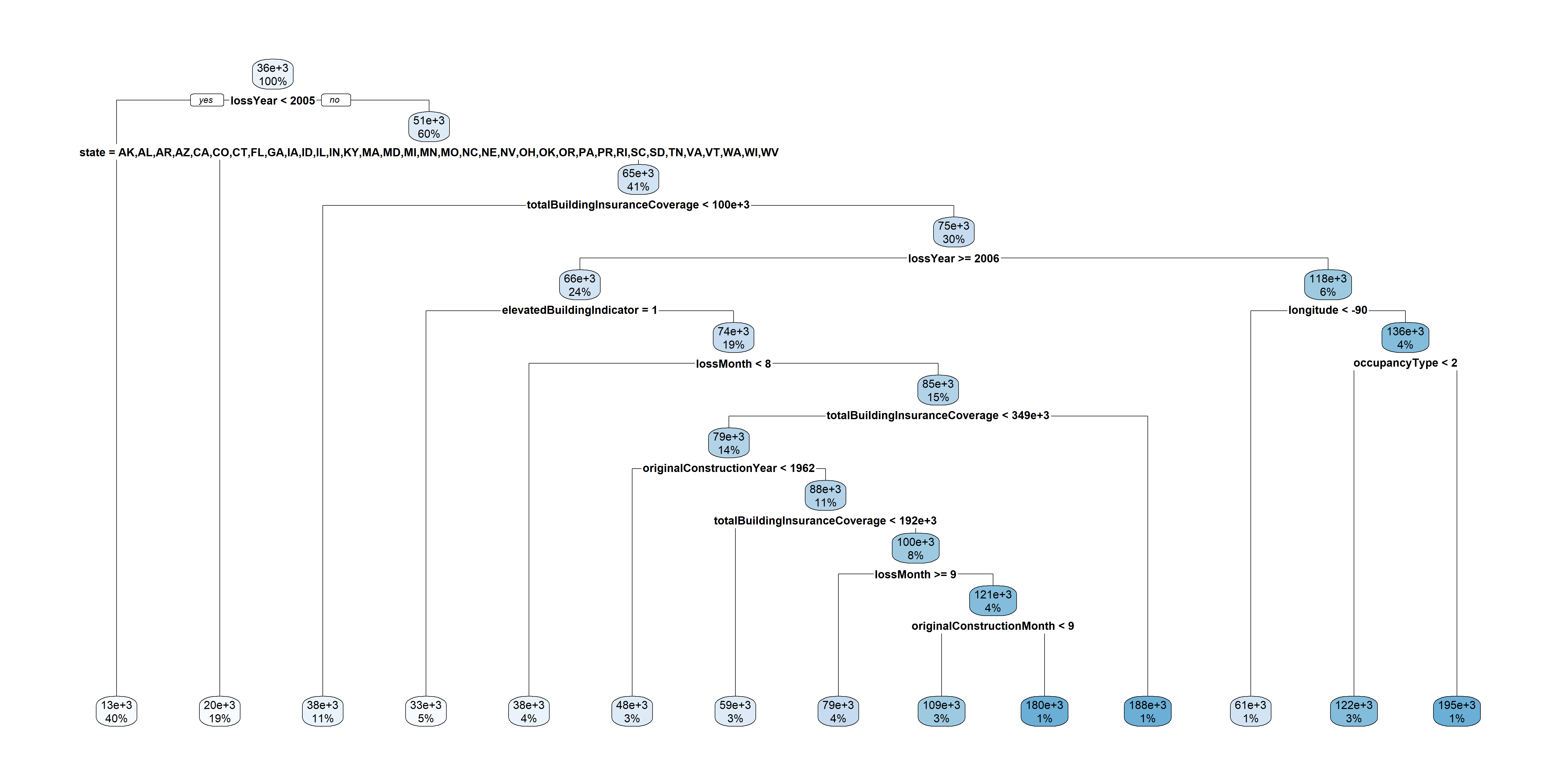
Plot claims by year
Plot average claim size by year
Number of claims by state
Prepare to make state-based maps for USA
claims$state_full <- state.name[match(claims$state, state.abb)]

state_claims <- claims %>%
  group_by(state_full) %>%
  summarise(num_claims = n(),
            max_claim_size = max(amountPaidOnBuildingClaim),
            common = num_claims >= nrow(claims) / 100)

claims$state_full <- NULL

# Merge with the map data
states_map <- map_data("state")
state_claims$region <- tolower(state_claims$state_full)
states_map <- left_join(states_map, state_claims, by = "region")
Code
ggplot(states_map, aes(long, lat, group = group, fill = num_claims)) +
  geom_polygon(color = "white") +
  scale_fill_viridis_c(option = "C") +
  labs(title = "Number of Claims by State",
       fill = "Number of Claims") +
  theme_minimal() +
  theme(axis.title = element_blank(), axis.text = element_blank(), axis.ticks = element_blank())
Max claim size by state
Code
# Plot maximum claim size by state
ggplot(states_map, aes(long, lat, group = group, fill = max_claim_size)) +
  geom_polygon(color = "white") +
  scale_fill_viridis_c(option = "C") +
  labs(title = "Maximum Claim Size by State",
       fill = "Max Claim Size") +
  theme_minimal() +
  theme(axis.title = element_blank(), axis.text = element_blank(), axis.ticks = element_blank())
Some states have very few claims
Code
# Plot states where floods are common
ggplot(states_map, aes(long, lat, group = group, fill = common)) +
  geom_polygon(color = "white") +
  scale_fill_viridis_d() +
  labs(title = "States where flood claims are frequent",
       fill = "Number of Claims >= 1%") +
  theme_minimal() +
  theme(axis.title = element_blank(), axis.text = element_blank(), axis.ticks = element_blank())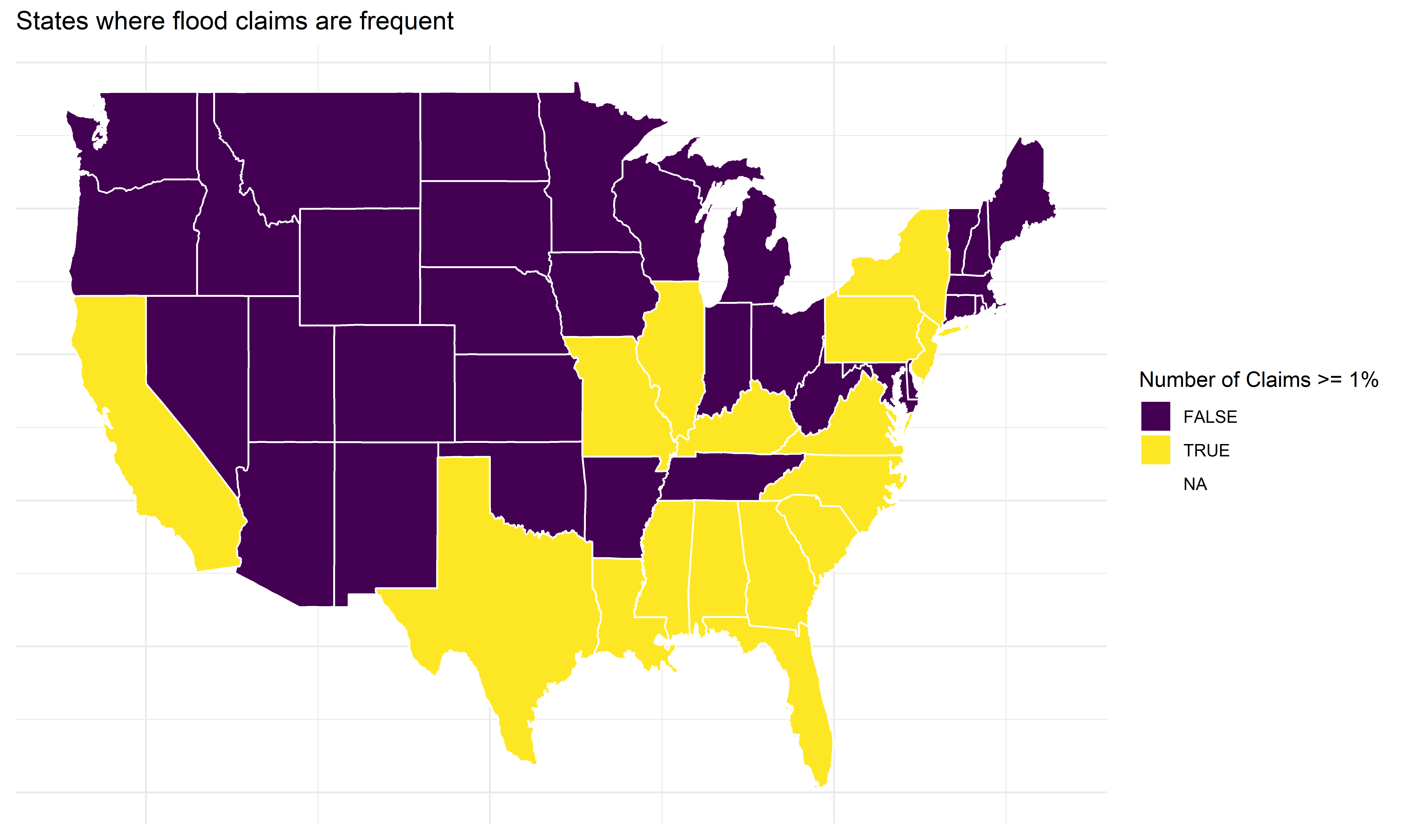
Geographical distribution of perils
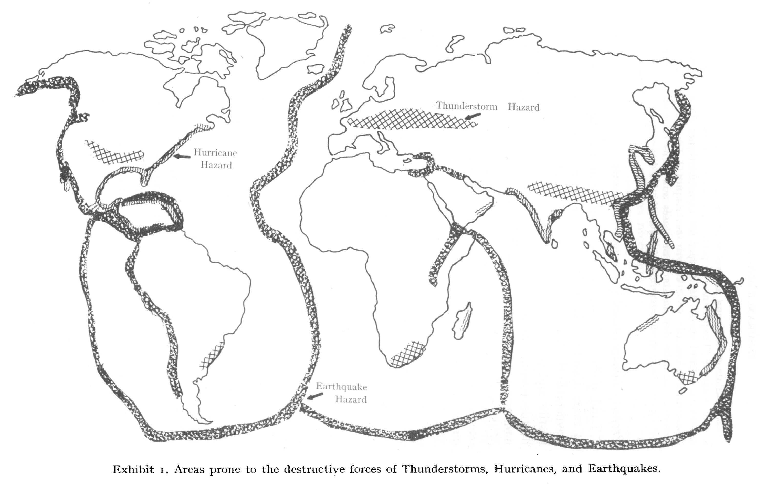
Friedman Exhibit 1 (p. 10).
Hot spots
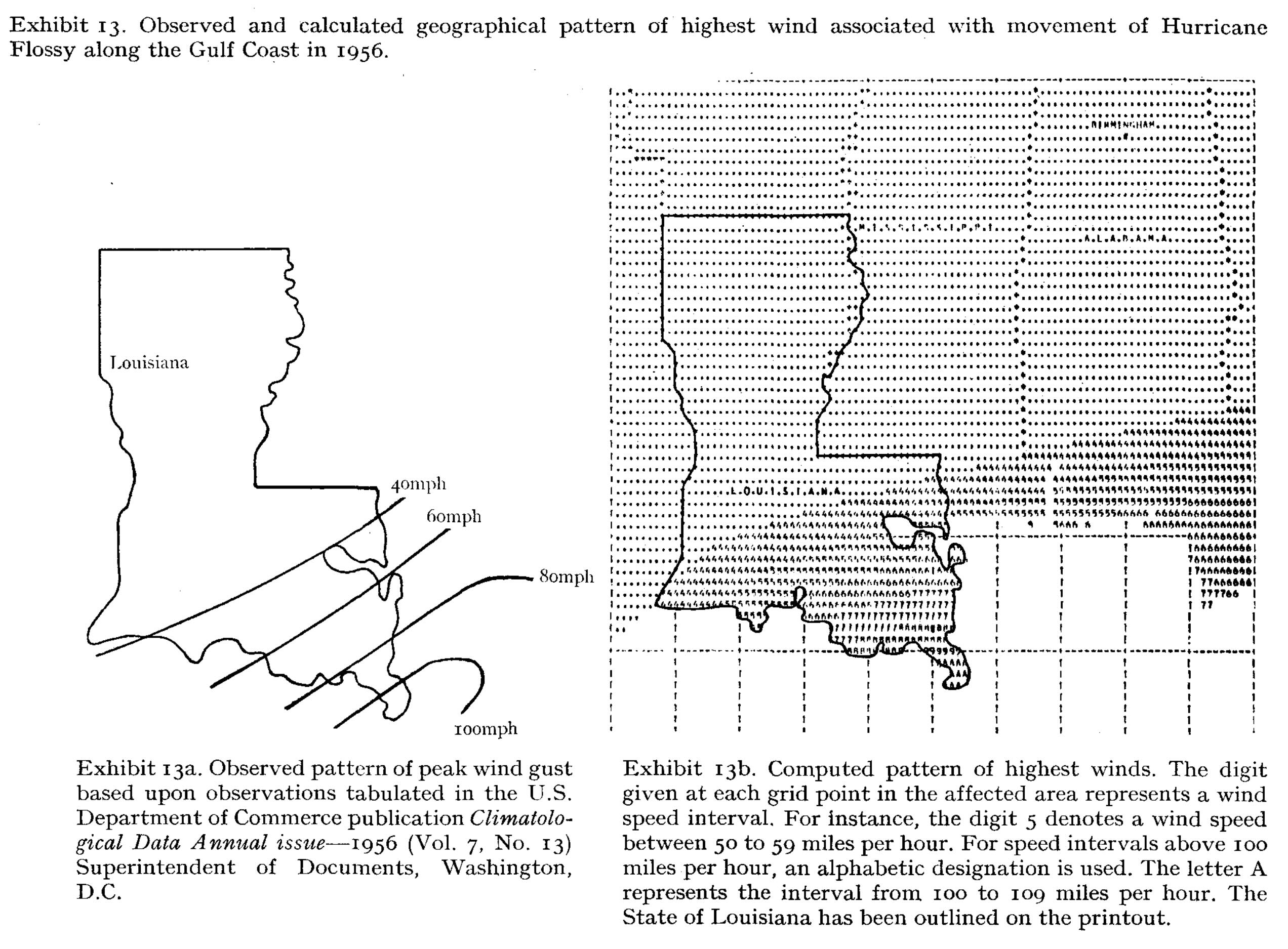
Friedman Exhibit 13 (p. 46).
New tree
More data
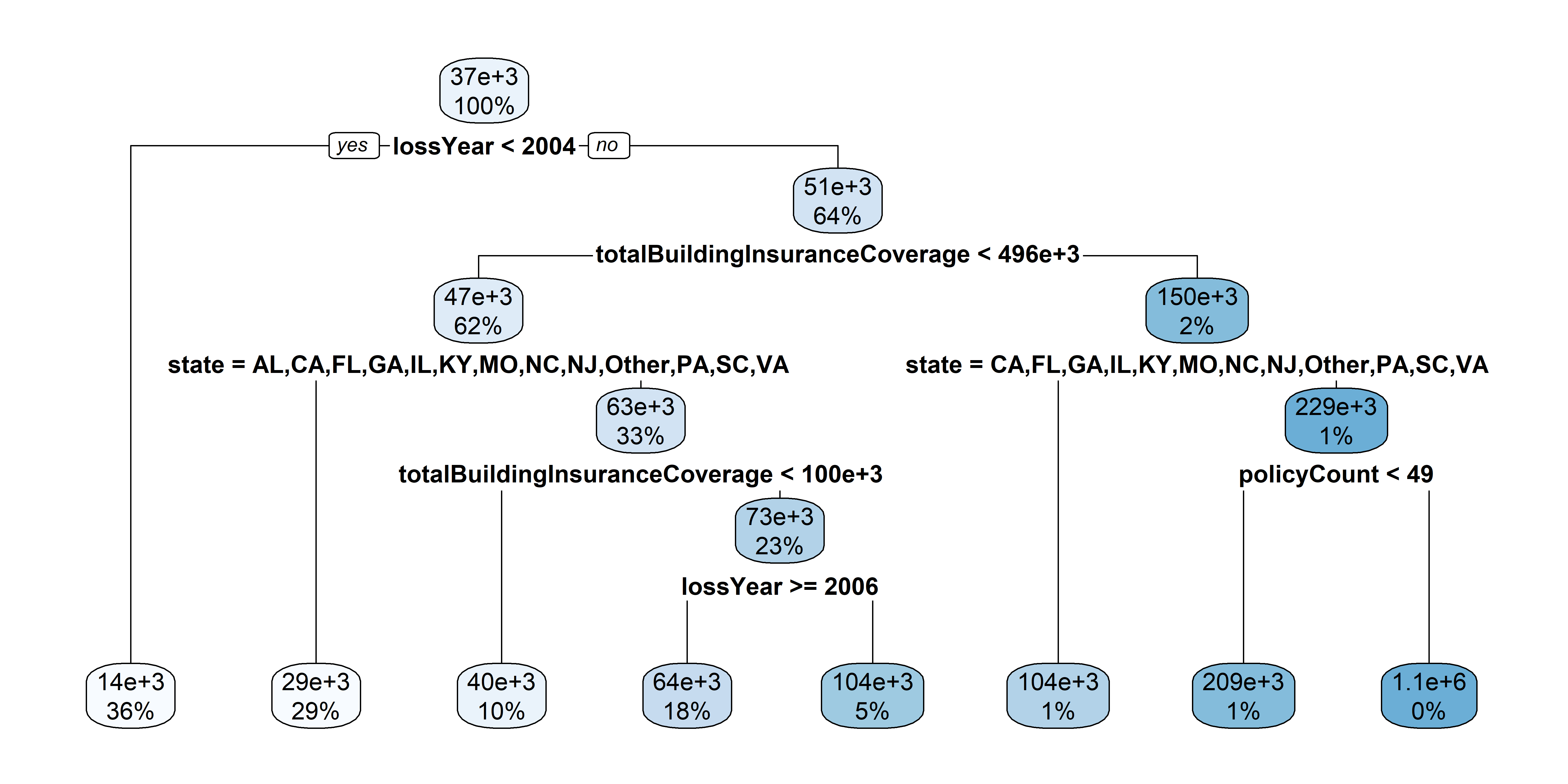
What’s the best size of tree
The smallest tree is just a root node (no splits).
The upper limit is to grow until one observation in each region.
How large should we grow the tree?
- What’s wrong if the tree is too small?
- What’s wrong if the tree is too large?

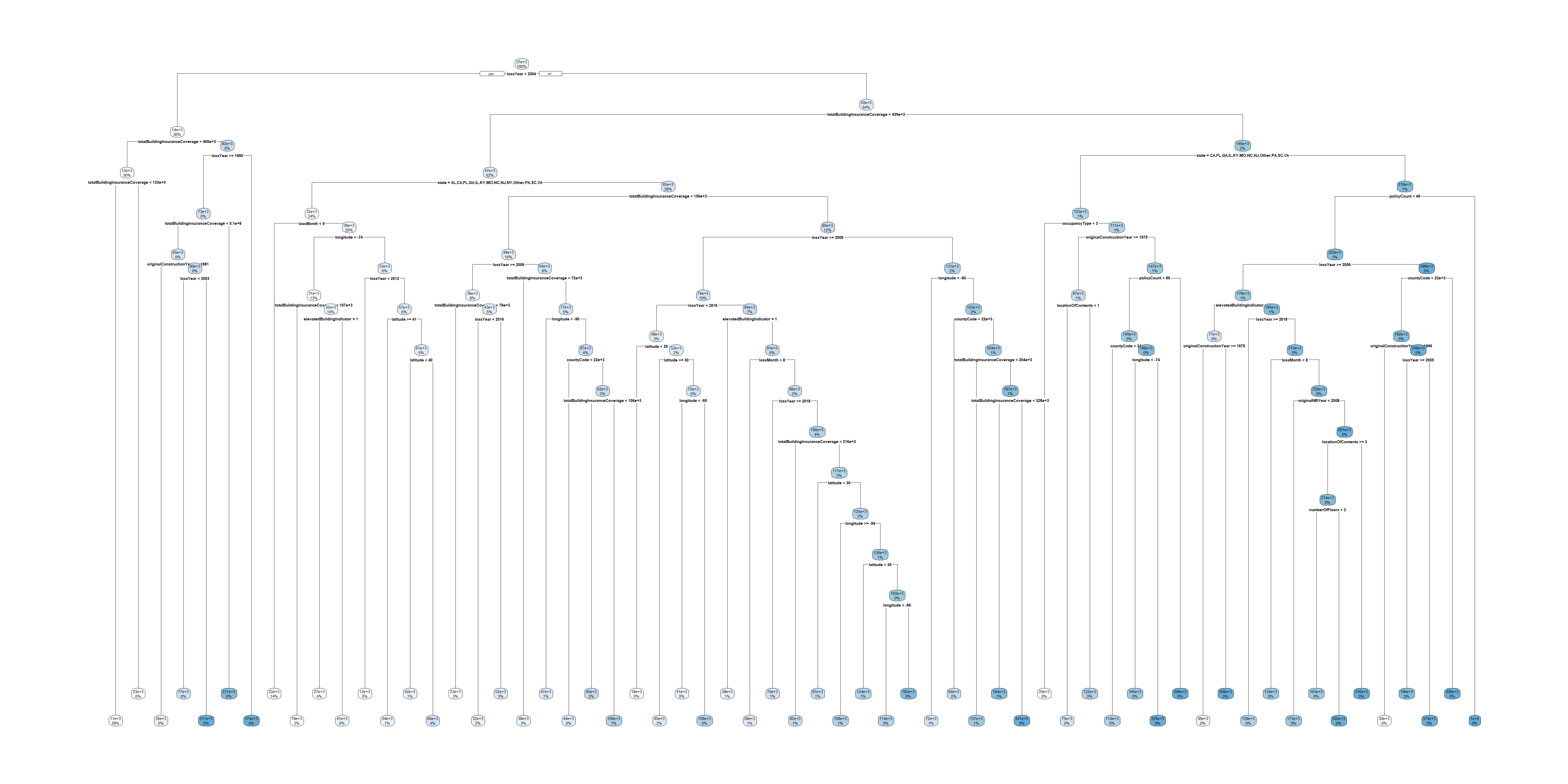
A large tree for the flood insurance data
Code
# I have already shuffled this data
train_val_index <- 1:(0.8*nrow(claims))
train_val_set <- claims[train_val_index, ]
test_set <- claims[-train_val_index, ]

train_index <- 1:(0.75*nrow(train_val_set))
train_set <- train_val_set[train_index, ]
val_set <- train_val_set[-train_index, ]

# train_set$rateMethod <- factor(train_set$rateMethod)
train_set$state <- factor(train_set$state)

# val_set$rateMethod <- factor(val_set$rateMethod, levels = levels(train_set$rateMethod))
val_set$state <- factor(val_set$state, levels = levels(train_set$state))

# test_set$rateMethod <- factor(test_set$rateMethod, levels = levels(train_set$rateMethod))
test_set$state <- factor(test_set$state, levels = levels(train_set$state))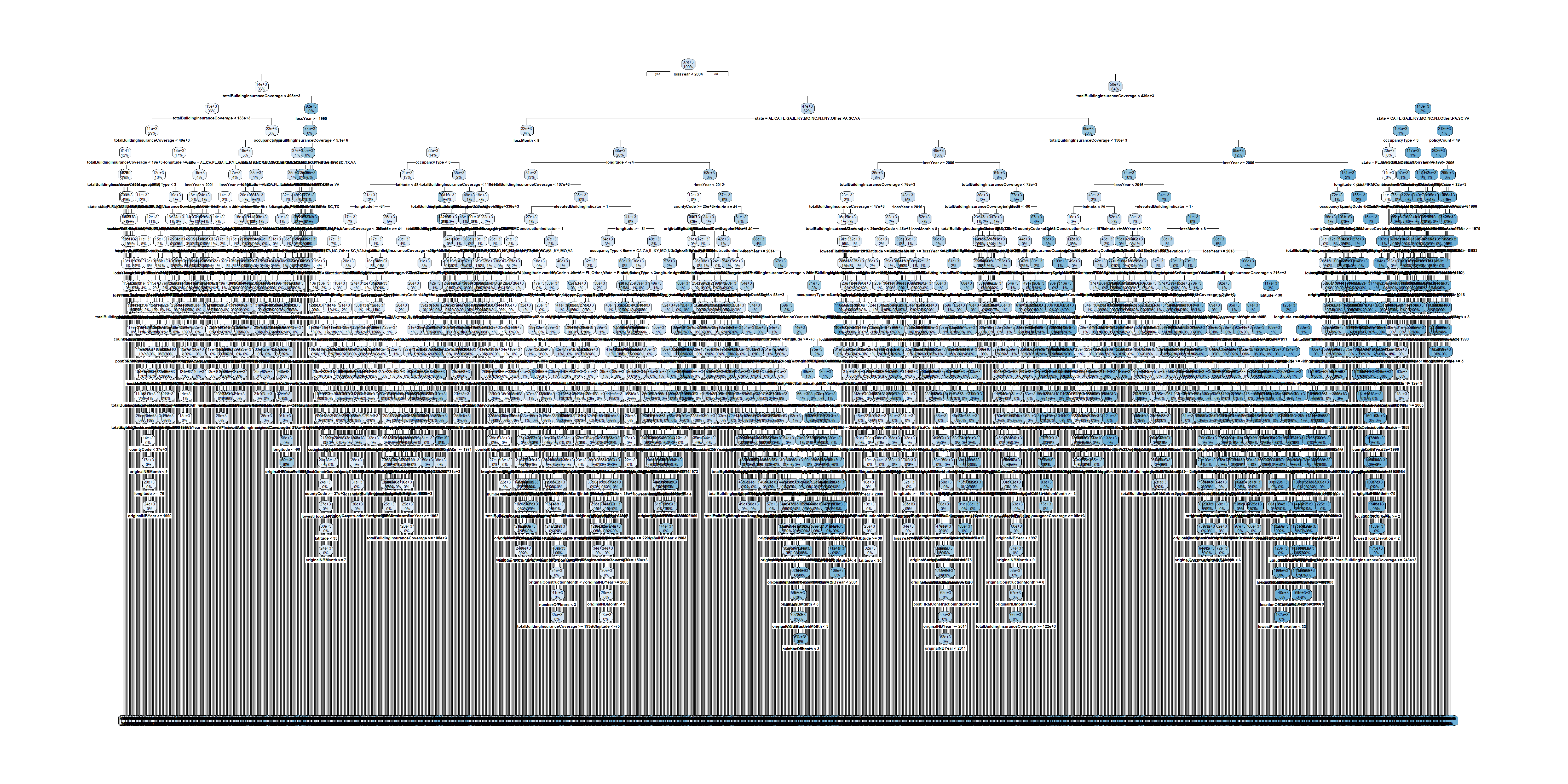
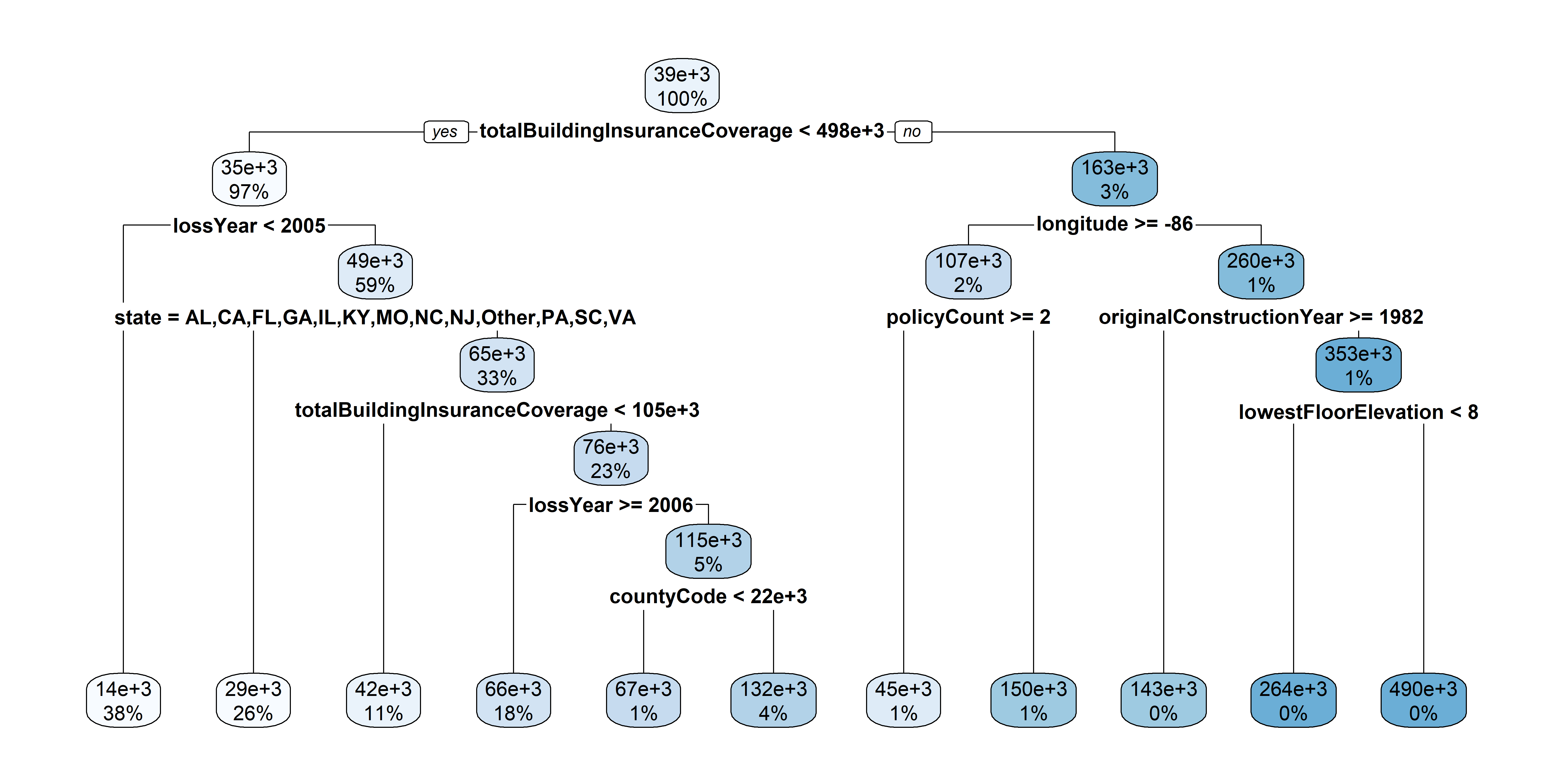
The full tree for train pricing
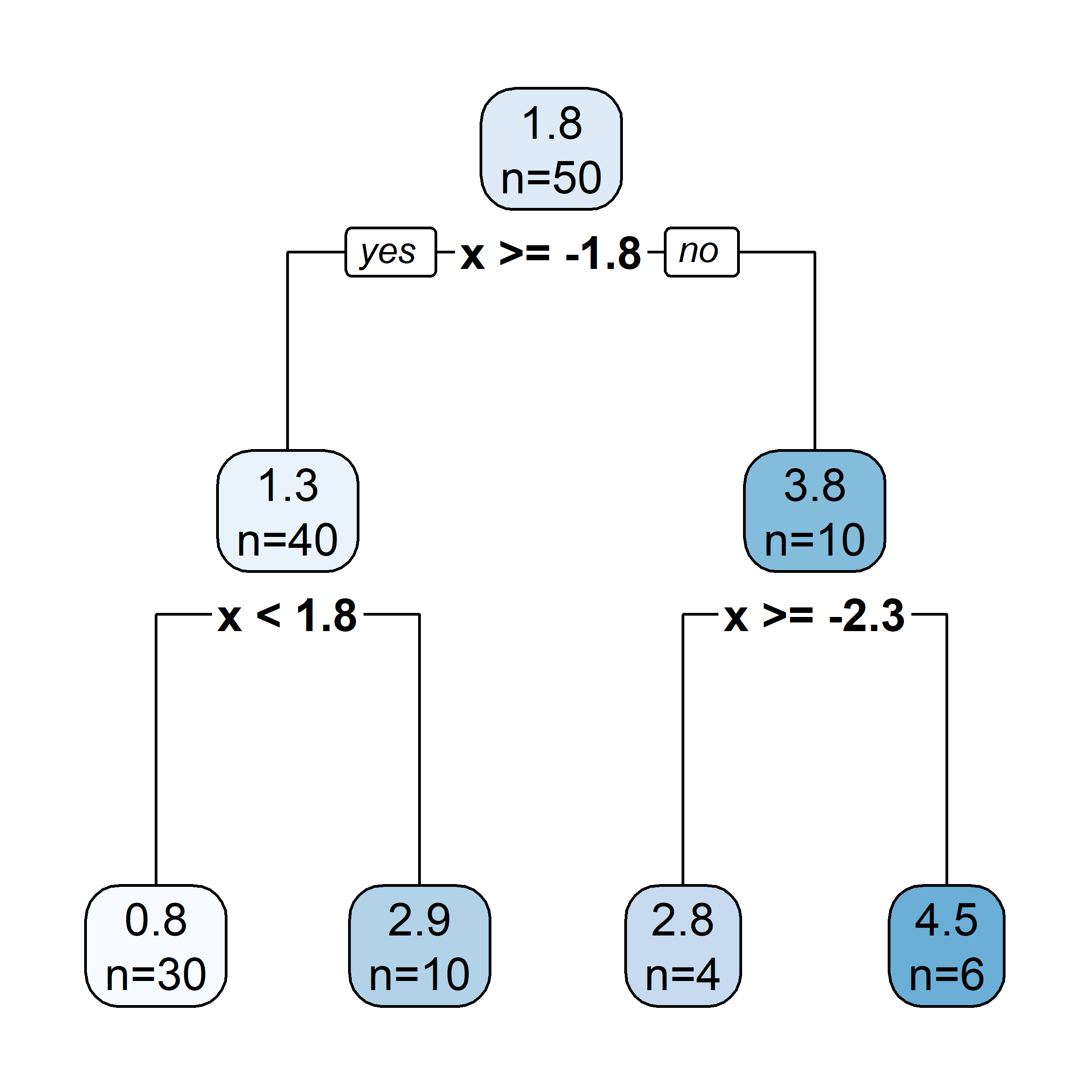
Unpruned Hitters tree: all predictors

The unpruned tree that results from top-down greedy splitting on the training data.
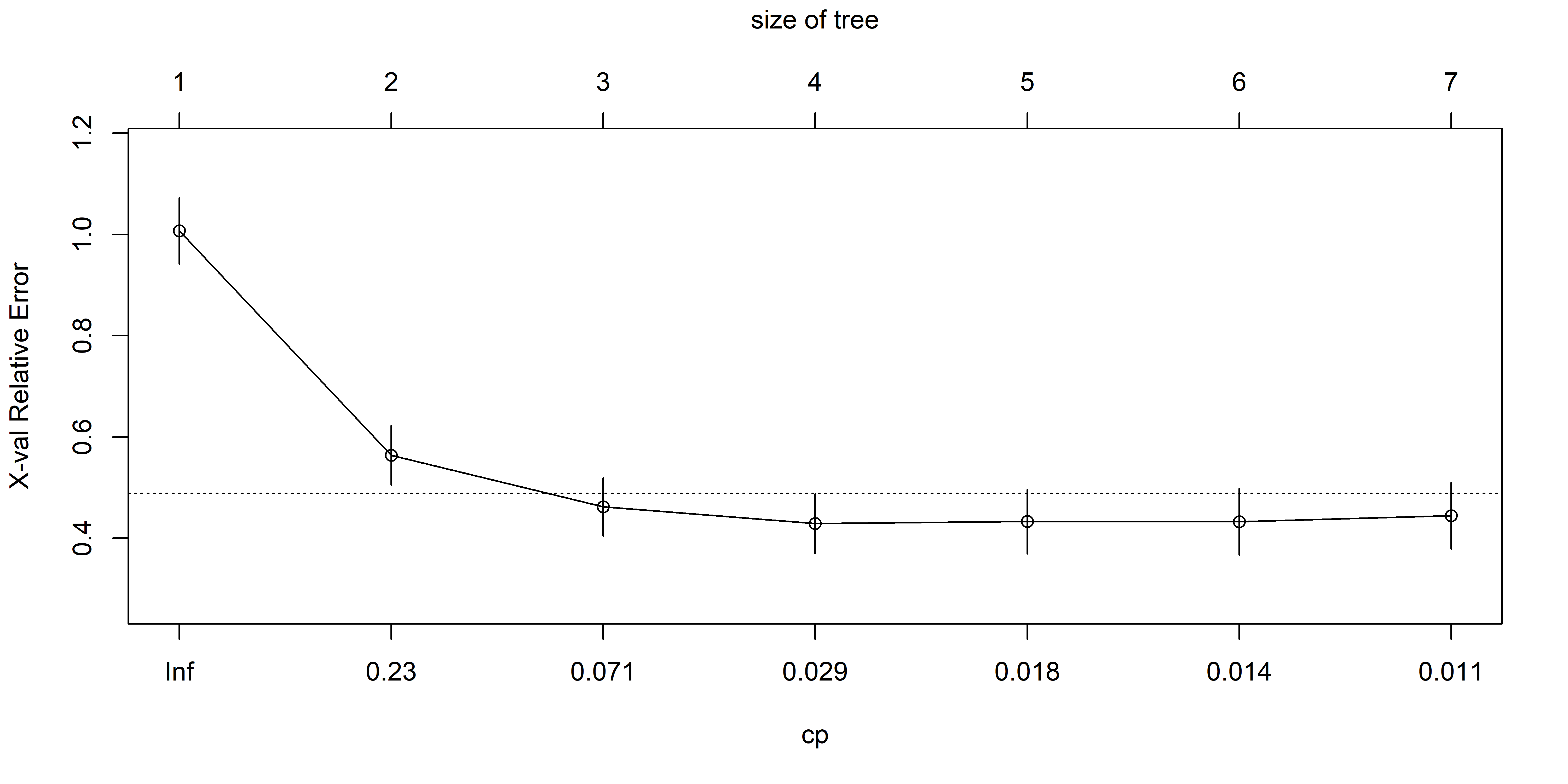
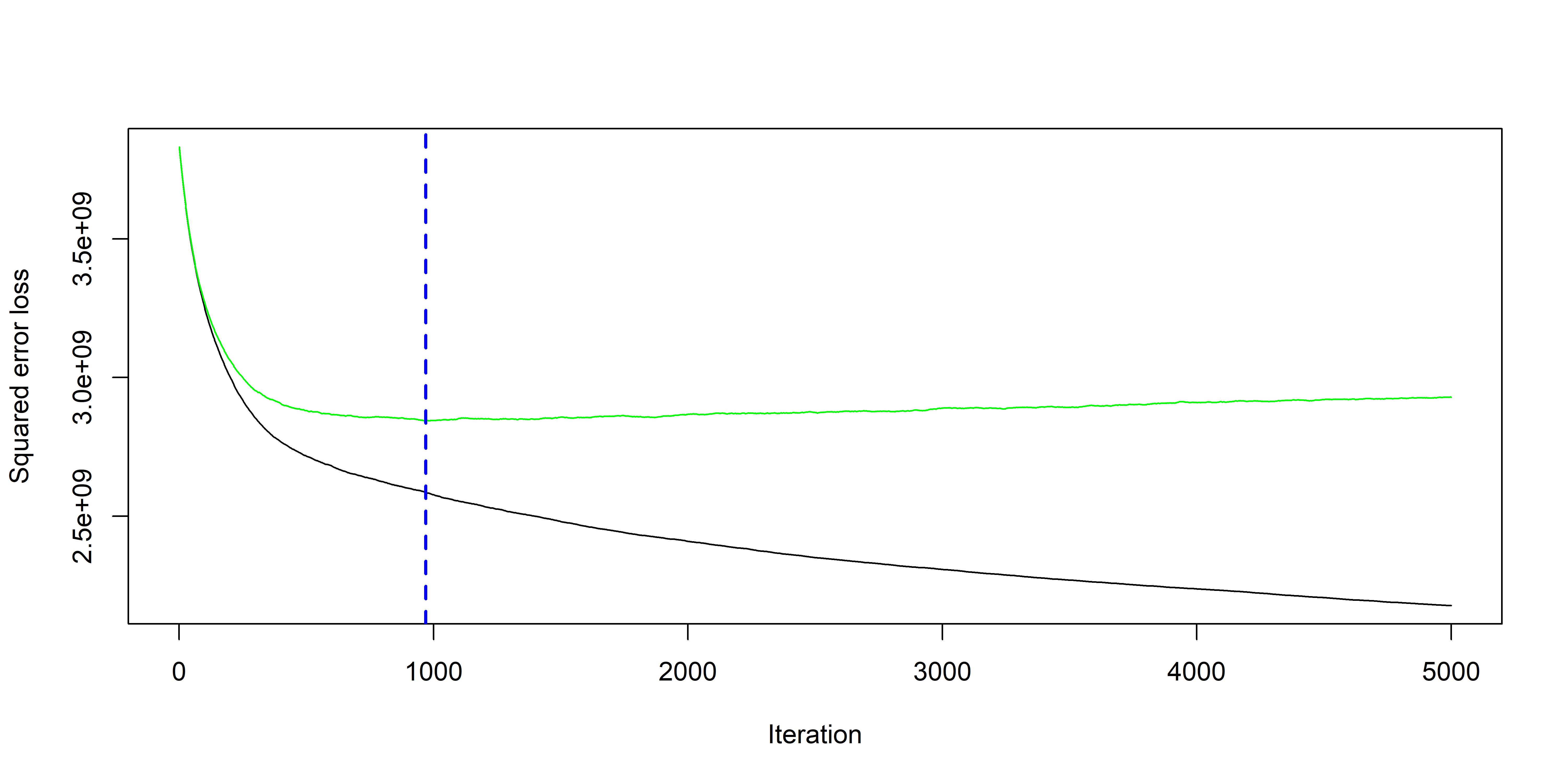
CV to pick \alpha (equiv., |T|)

The training, cross-validation, and test MSE are shown as a function of the number of terminal nodes in the pruned tree. Standard error bands are displayed. The minimum cross-validation error occurs at a tree of size three.
CV to prune NFIP tree
Cross-validation to prune the large NFIP tree
# Perform cross-validation to prune the tree
set.seed(123)
cv_tree <- train(
  amountPaidOnBuildingClaim ~ .,
  data=train_set,
  method="rpart",
  trControl=trainControl(method="cv", number=5),
  tuneGrid=data.frame(cp=seq(0, 0.01, 0.001))
)
# Get the optimal cp value
optimal_cp <- cv_tree$bestTune$cp
plot(cv_tree)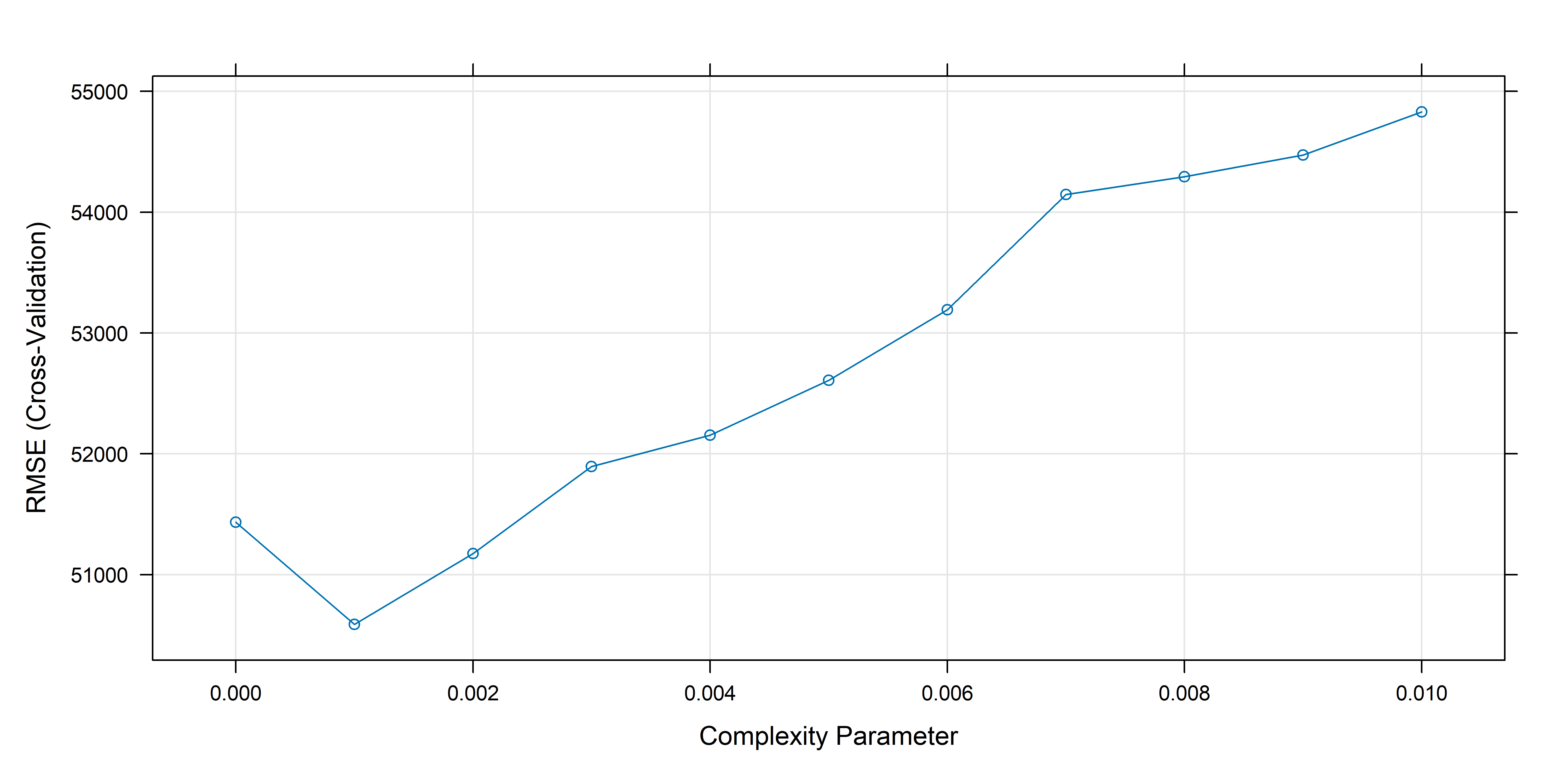
The pruned tree
An ensemble is a group of models…
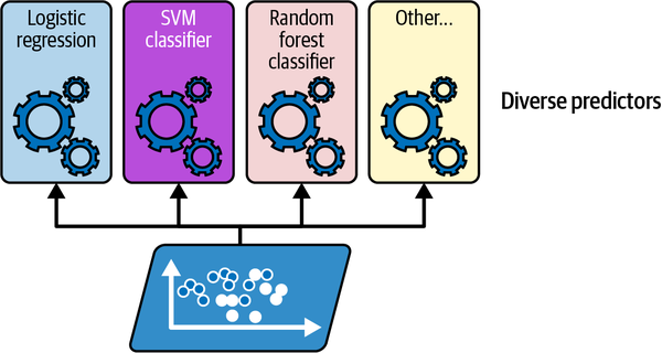
Training various different classifiers on the same dataset.
… & you combine their predictions
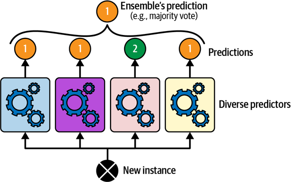
Make an overall prediction based on the majority vote of the models.
Bootstrapping
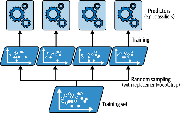
Train on different versions of the same data.
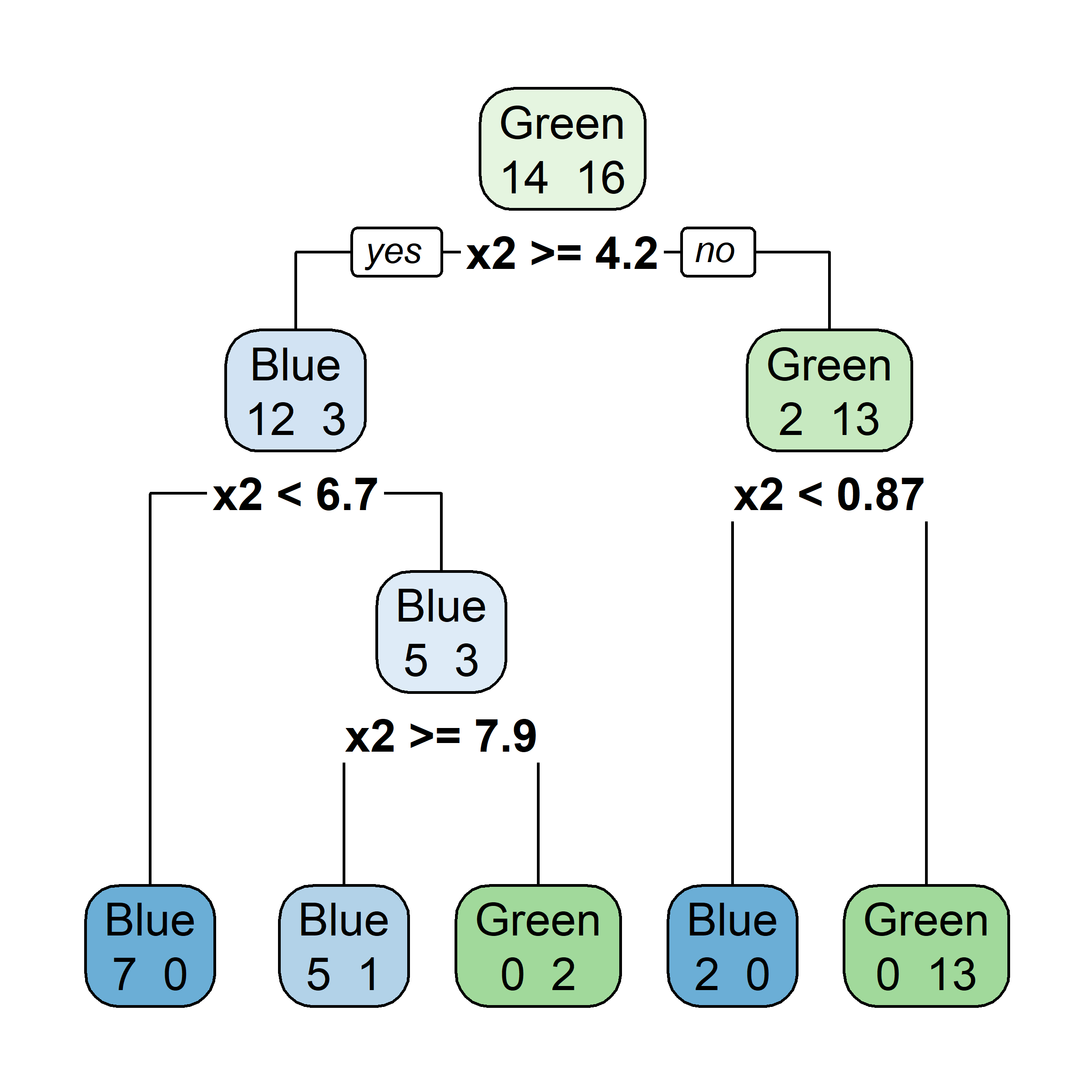
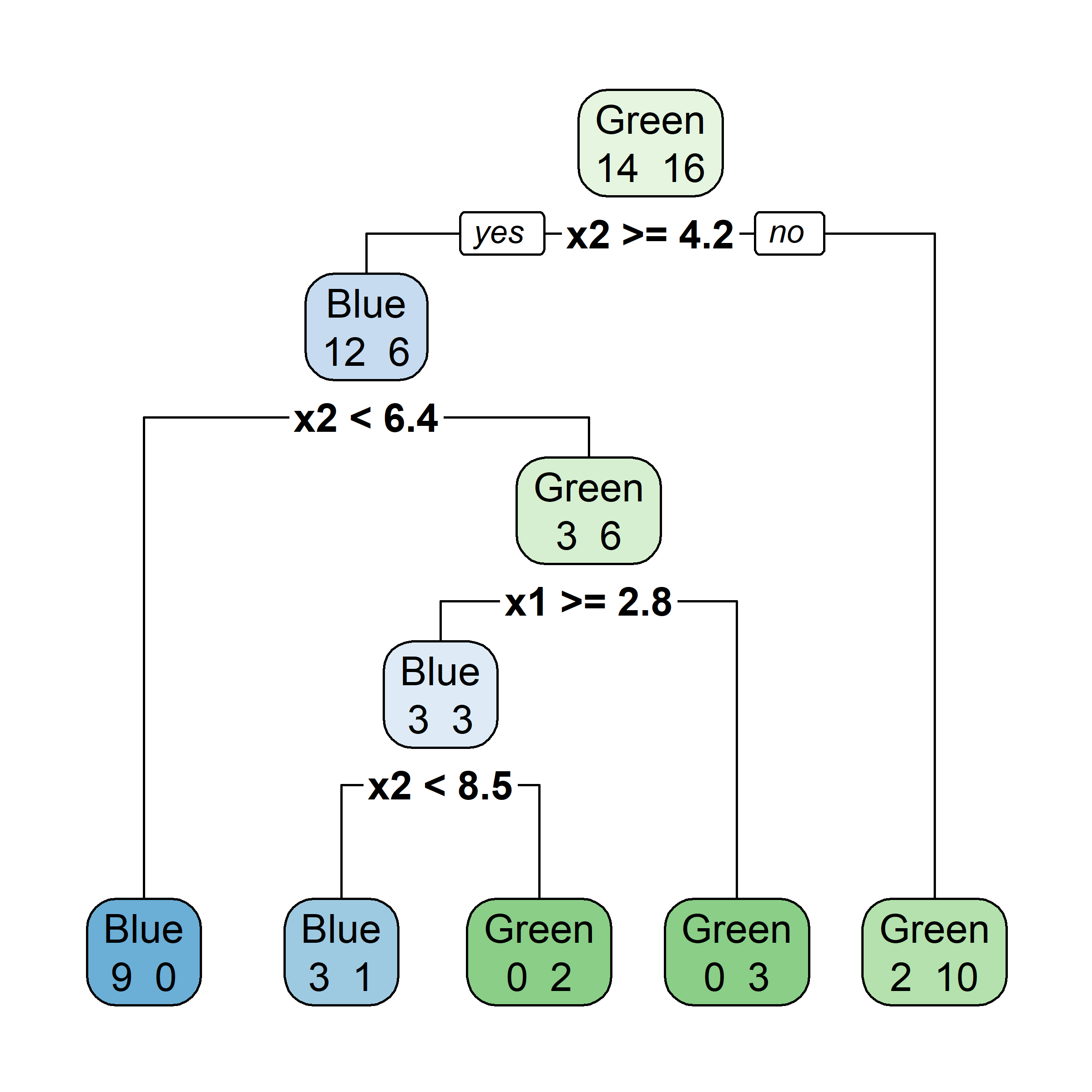
Bagging: Illustration
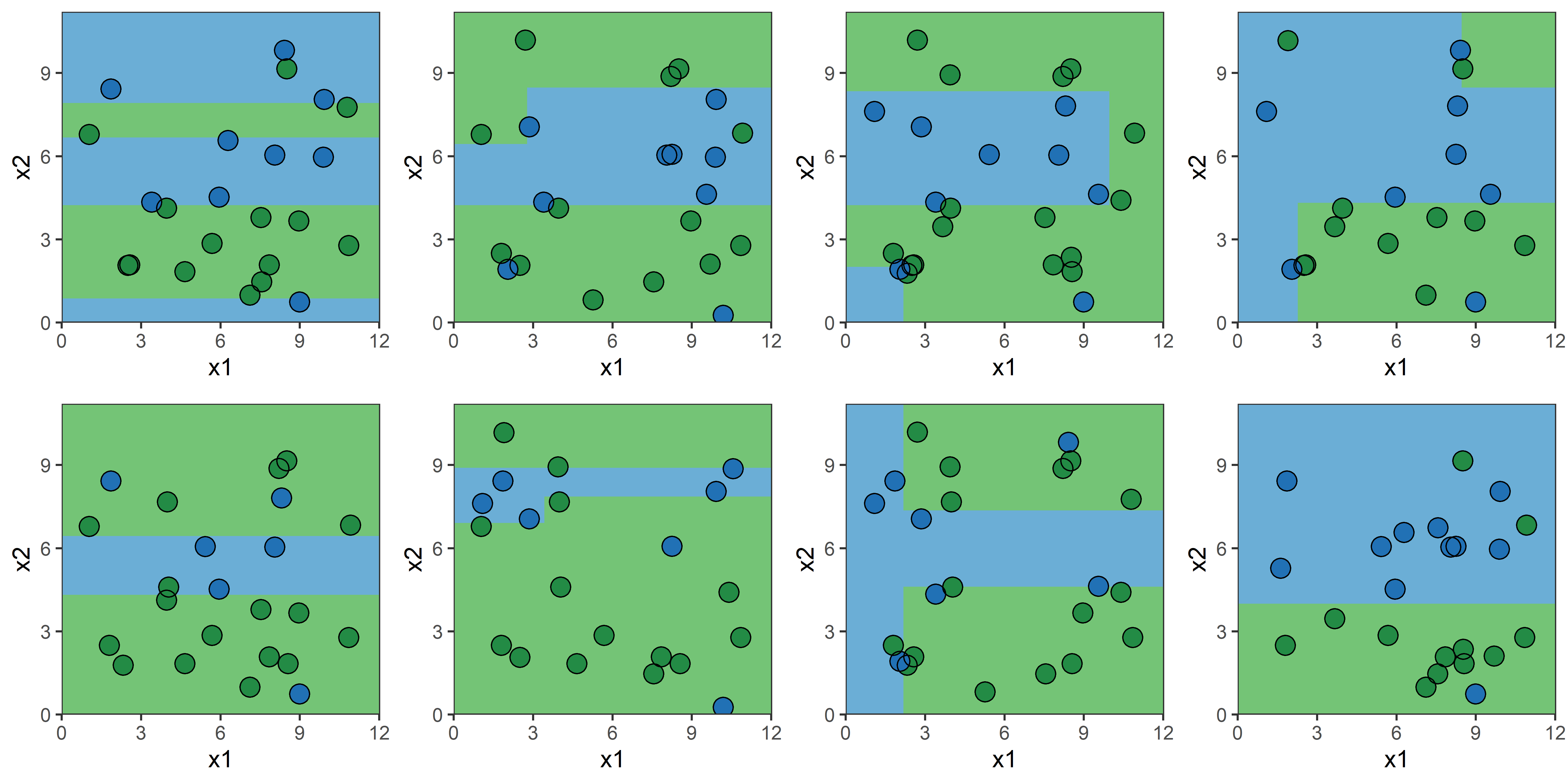
Bagging: Illustration
Random Forests

This is a forest (stock photo)
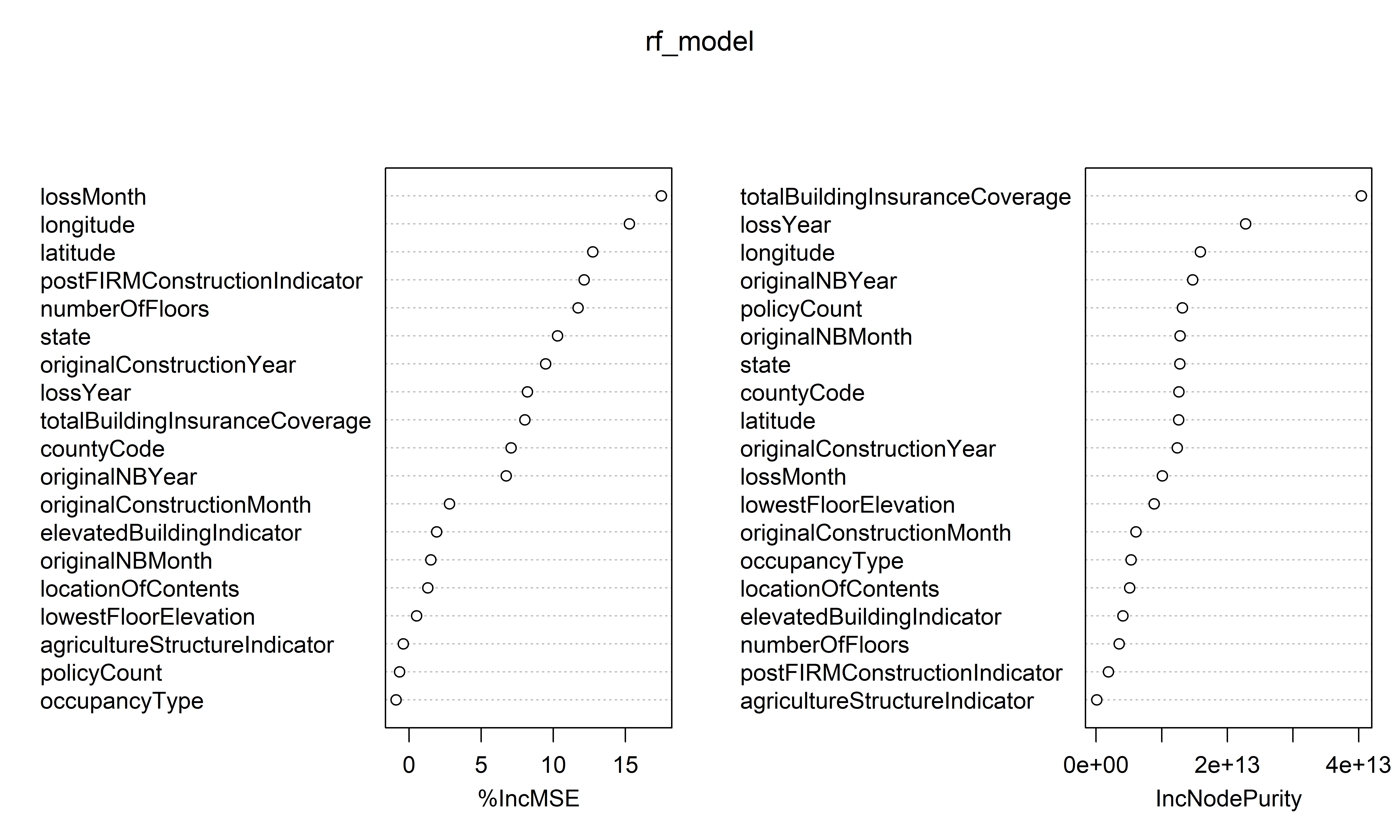
Variable importance plot
Fitting with package gbm
Boosting (iteration 1)
Code
x_obs = np.linspace(-3, 3, 50)
y_obs = [5, 4, 5, 4, 5, 4, 1, 2, 4, 4, 2, 1, 2, 1, 1, 1, 2, 0, 0, 0, 2, 0, 1, 1, 1, 0, 1, 1, -1, 1, 0, 1, 0, -1, 2, 0, 1, 2, 1, 1, 3, 2, 4, 1, 2, 2, 4, 3, 5, 3]
df = pd.DataFrame({'x': x_obs, 'y': y_obs})

# Parameters
d = 1  # number of splits
lambda_ = 0.5  # learning rate

# Higher resolution grid
x_obs = x_obs.reshape(-1, 1)
x_grid = np.linspace(-3, 3, 1000)

# Initial model
f_hat = np.zeros_like(df['y'], dtype=float)
residuals = df['y'].astype(float).copy()

# Store predictions for the grid
f_hat_grid = np.zeros_like(x_grid, dtype=float)

def plot_boosting_iteration(df, x_grid, f_hat, residuals, f_hat_grid, d, lambda_):
  fig, axes = plt.subplots(1, 3, figsize=(10, 4))

  # Plot residuals
  axes[0].scatter(df['x'], residuals, color='blue', label='Residuals')
  axes[0].plot(x_grid, f_b_grid, color='green', label='New Tree')
  axes[0].set_ylim(-1.25, 5.25)
  axes[0].set_title(f"Residuals")

  # Plot updated model prediction
  axes[1].plot(x_grid, f_hat_grid, color='purple')
  axes[1].scatter(df['x'], df['y'], color='red', alpha=0.5)
  axes[1].set_ylim(-1.25, 5.25)
  axes[1].set_title(f"Updated Prediction")

  # Plot new residuals
  axes[2].scatter(df['x'], df['y'] - f_hat, color='blue', label='Residuals')
  axes[2].set_ylim(-1.25, 5.25)
  axes[2].set_title(f"New Residuals")

  plt.tight_layout()
Code
# Fit a tree to residuals
tree = DecisionTreeRegressor(max_depth=d)
tree.fit(x_obs, residuals);
f_b = tree.predict(x_obs)
f_b_grid = tree.predict(x_grid.reshape(-1, 1))

# Update model
f_hat += lambda_ * f_b
f_hat_grid += lambda_ * f_b_grid
plot_boosting_iteration(df, x_grid, f_hat, residuals, f_hat_grid, d, lambda_)

# Update residuals
residuals -= lambda_ * f_b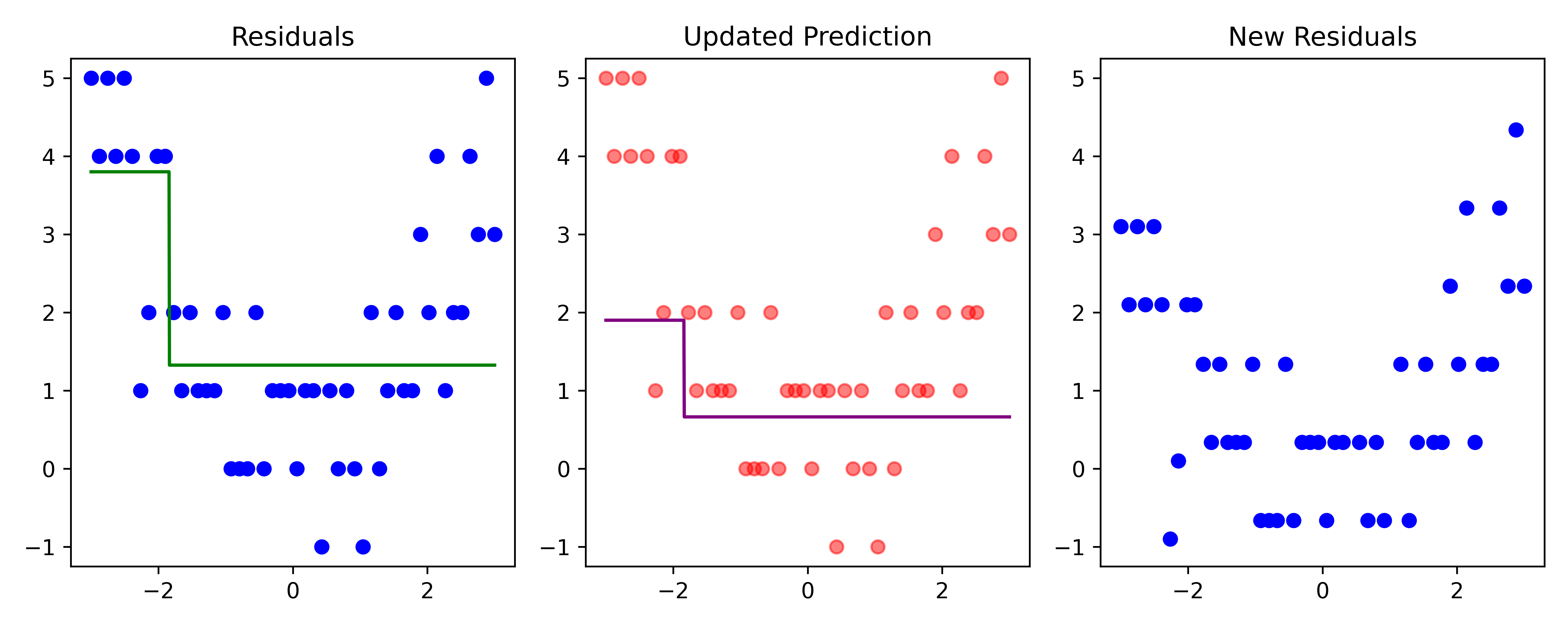
Here, \lambda=\frac12 is the learning rate.
Boosting (iteration 2)
Code
# Fit a tree to residuals
tree = DecisionTreeRegressor(max_depth=d)
tree.fit(x_obs, residuals);
f_b = tree.predict(x_obs)
f_b_grid = tree.predict(x_grid.reshape(-1, 1))

# Update model
f_hat += lambda_ * f_b
f_hat_grid += lambda_ * f_b_grid
plot_boosting_iteration(df, x_grid, f_hat, residuals, f_hat_grid, d, lambda_)

# Update residuals
residuals -= lambda_ * f_b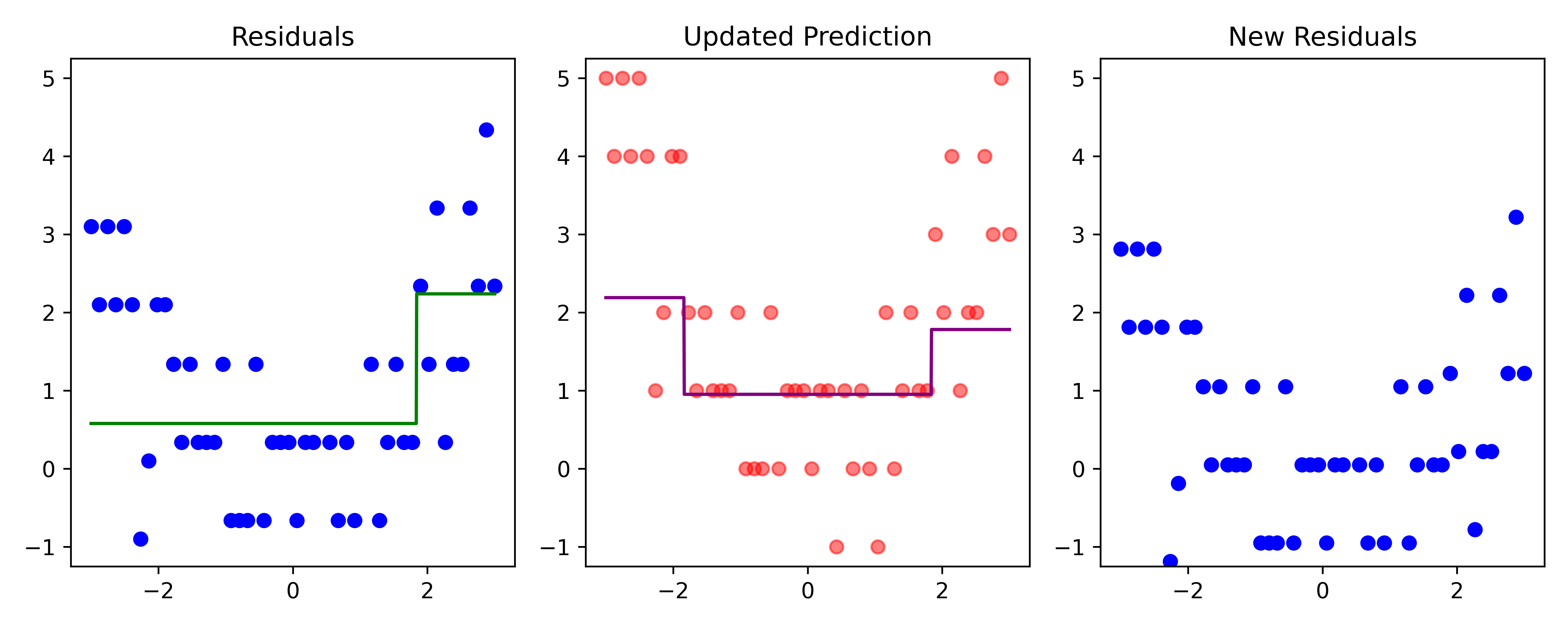
Here, \lambda=\frac12 is the learning rate.
Boosting (iteration 3)
Code
# Fit a tree to residuals
tree = DecisionTreeRegressor(max_depth=d)
tree.fit(x_obs, residuals);
f_b = tree.predict(x_obs)
f_b_grid = tree.predict(x_grid.reshape(-1, 1))

# Update model
f_hat += lambda_ * f_b
f_hat_grid += lambda_ * f_b_grid
plot_boosting_iteration(df, x_grid, f_hat, residuals, f_hat_grid, d, lambda_)

# Update residuals
residuals -= lambda_ * f_b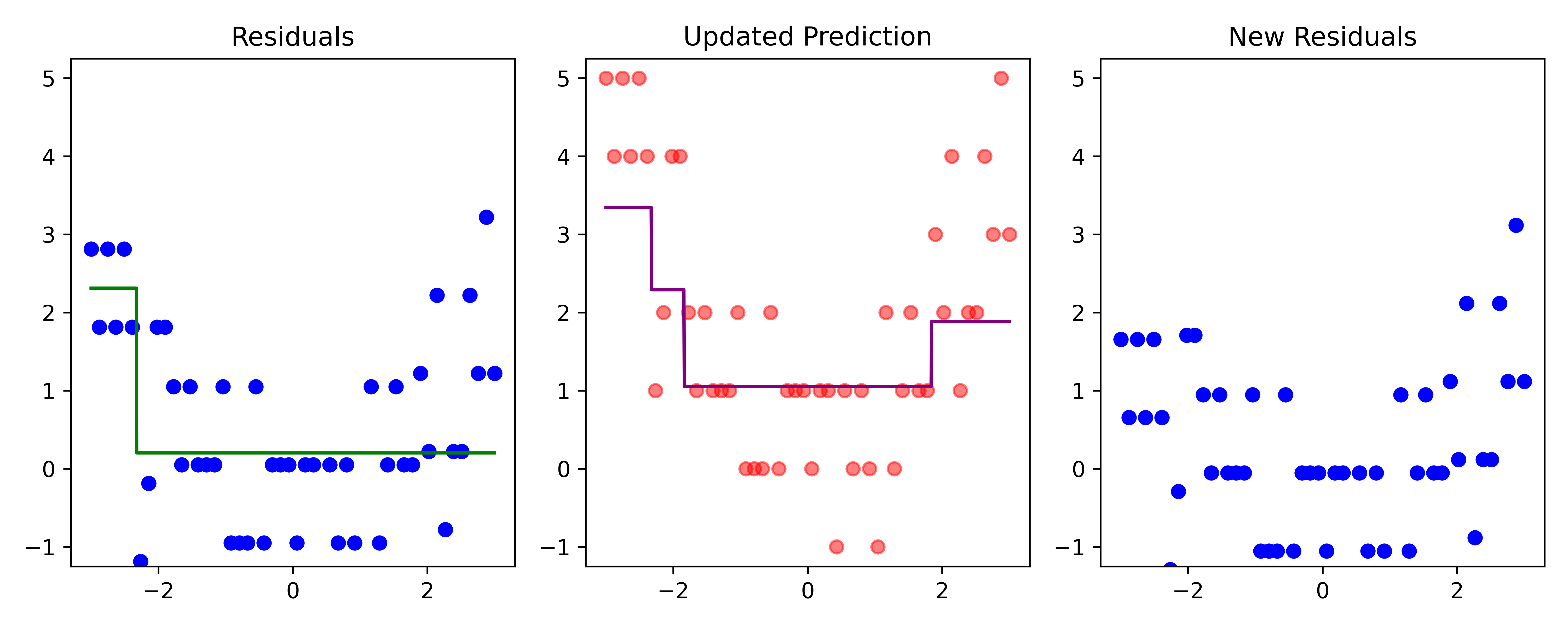
Here, \lambda=\frac12 is the learning rate.
Boosting (iteration 4)
Code
# Fit a tree to residuals
tree = DecisionTreeRegressor(max_depth=d)
tree.fit(x_obs, residuals);
f_b = tree.predict(x_obs)
f_b_grid = tree.predict(x_grid.reshape(-1, 1))

# Update model
f_hat += lambda_ * f_b
f_hat_grid += lambda_ * f_b_grid
plot_boosting_iteration(df, x_grid, f_hat, residuals, f_hat_grid, d, lambda_)

# Update residuals
residuals -= lambda_ * f_b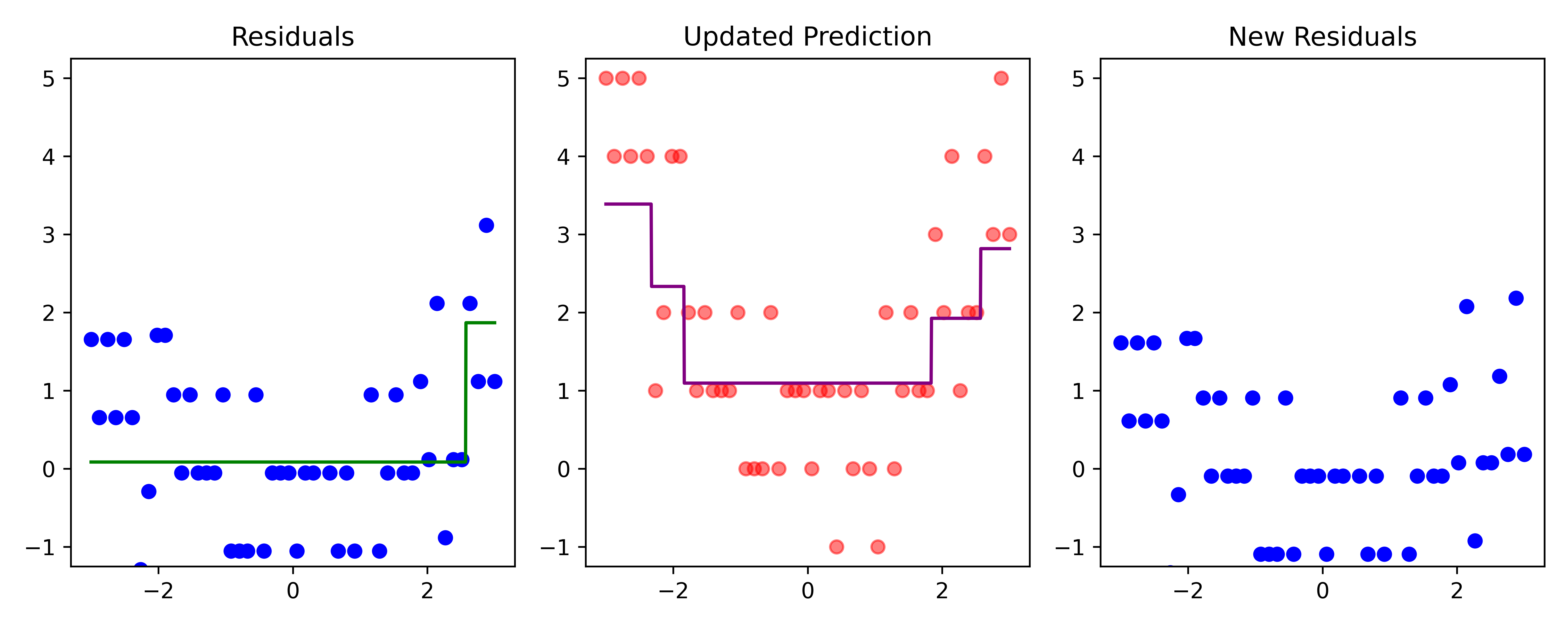
Here, \lambda=\frac12 is the learning rate.
Boosting (iteration 5)
Code
# Fit a tree to residuals
tree = DecisionTreeRegressor(max_depth=d)
tree.fit(x_obs, residuals);
f_b = tree.predict(x_obs)
f_b_grid = tree.predict(x_grid.reshape(-1, 1))

# Update model
f_hat += lambda_ * f_b
f_hat_grid += lambda_ * f_b_grid
plot_boosting_iteration(df, x_grid, f_hat, residuals, f_hat_grid, d, lambda_)

# Update residuals
residuals -= lambda_ * f_b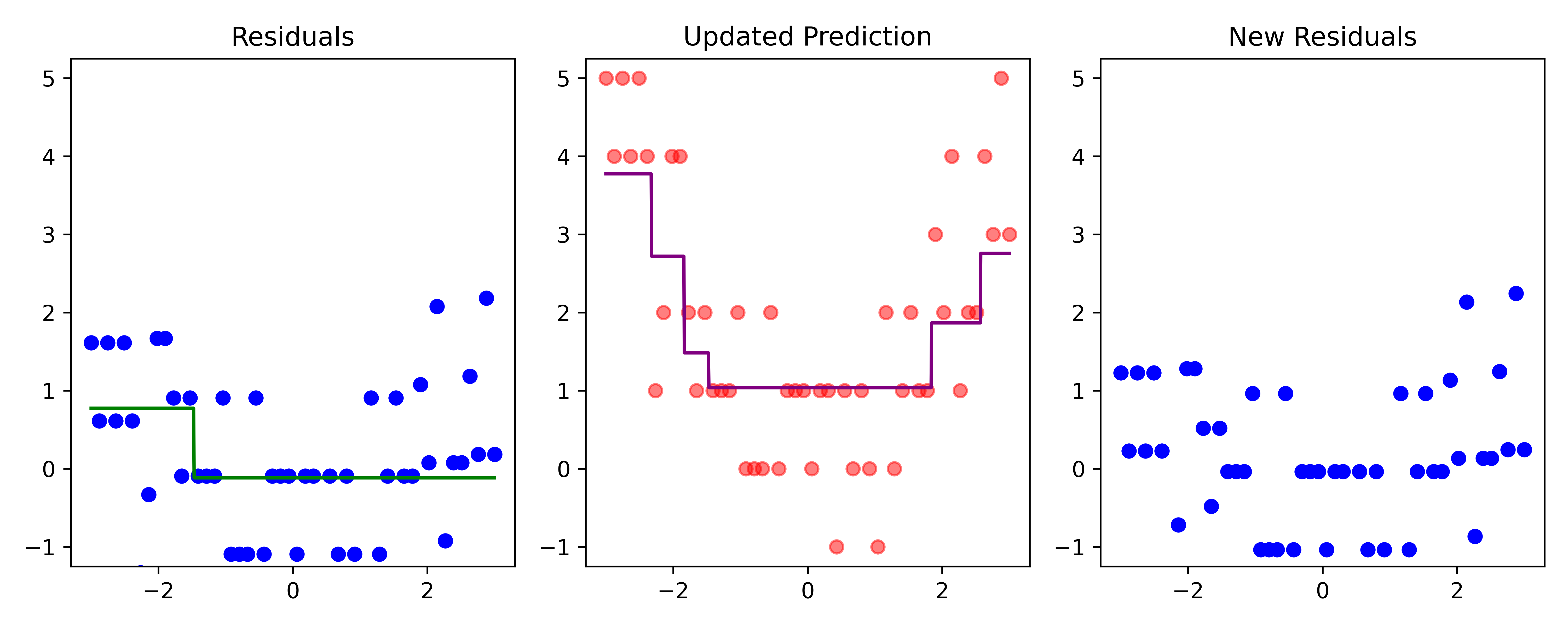
Here, \lambda=\frac12 is the learning rate.
Sensitivity to training data orientation
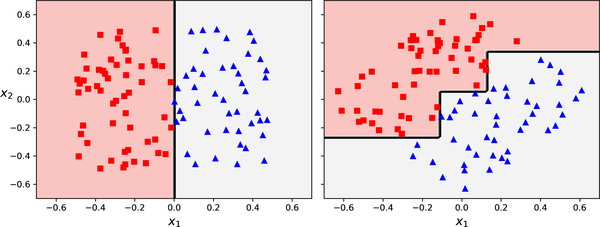
An example of a dataset which is rotated and fit to decision trees.