(myVector <- c(7,11,13)) # Create a vector called 'myVector'[1] 7 11 13myVector * 3[1] 21 33 39myVector[1] # Get the first element[1] 7myVector[3] # Get the third element[1] 13By the end of this topic, you should be able to
(myVector <- c(7,11,13)) # Create a vector called 'myVector'[1] 7 11 13myVector * 3[1] 21 33 39myVector[1] # Get the first element[1] 7myVector[3] # Get the third element[1] 13length(): returns the length of a vector.sort(): sorts the elements of a vector, in increasing or decreasing order.rev(): rearranges the elements of a vector in reverse order.rank(): returns the vector of ranks of the elements.head(): returns the first few elements of a vector.tail(): returns the last few elements of a vector.x <- c(1,3,6,2,7,4,8,1,0,8)
length(x)[1] 10sort(x) [1] 0 1 1 2 3 4 6 7 8 8sort(x, decreasing=TRUE) [1] 8 8 7 6 4 3 2 1 1 0rev(x) [1] 8 0 1 8 4 7 2 6 3 1rank(x) [1] 2.5 5.0 7.0 4.0 8.0 6.0 9.5 2.5 1.0 9.5head(x, 3)[1] 1 3 6tail(x, 2)[1] 0 8Note: The largest value of rank(x) is not always equal to length(x), as there could be a tie of largest values.
R allows for set operations on vectors
A <- c(4,5,2,7)
B <- c(2,1,7)
intersect(A,B)
[1] 2 7union(A,B)[1] 4 5 2 7 1setdiff(A,B)[1] 4 5setdiff(B,A)[1] 1is.element(A,B)[1] FALSE FALSE TRUE TRUEis.element(B,A)[1] TRUE FALSE TRUEBecause is.element is used often, R also provides a special operator %in% as shorthand:
4 %in% A[1] TRUEA %in% B[1] FALSE FALSE TRUE TRUEGiven that
A <- c(4,5,2,7)
B <- c(2,1,7,3)
C <- c(2,3,7)
Calculate
union(setdiff(A,B), setdiff(B,A))[1] 4 5 1 3length(intersect(intersect(A,B), C))[1] 2We saw before that to extract the ith element of a vector, we write myVector[i]. This is called indexing.
There are more methods for indexing which often prove useful:
vec <- c(2,5,6,8,10)
vec[c(2,3,4)] # Gets the 2nd, 3rd and 4th elements
[1] 5 6 8vec[2:4] # Does the same but in shorter notation[1] 5 6 8vec[-3] # Gets all elements *except* the 3rd[1] 2 5 8 10vec[-c(1,5)] # Gets all elements *except* the 1st and 5th[1] 5 6 8There is another extremely useful way of extracting from vectors which is ‘logical masks’. This works by specifying whether each element will be extracted using logical values.
vec[1] 2 5 6 8 10vec[c(T, F, T, T, F)] # Any index with T (for TRUE) gets returned[1] 2 6 8The above shows that any index with T gets returned. It is a somewhat contrived example because we must specify T/F for each index. Logical masks are more useful in situations as this one:
vec[vec > 5] [1] 6 8 10Indeed, we easily extracted all elements greater than 5 from vec, effectively “filtering” it.
x = c(1, 9, 0, 0, -5, 9, -5)
which(x == 0) # returns indices which satisfy the condition
[1] 3 4which.max(x) # returns the index of the *first* occurrence of the maximum[1] 2which.min(x) # returns the index of the *first* occurrence of the minimum value[1] 5which(x == min(x)) # same as which.min, but it returns *all* that satisfy the condition[1] 5 7name=c("Adam", "Bob", "Caitlin", "Josephine", "Jinxia")
height=c(165,182,178,160,155)
weight=c(50,85,67,55,48)
income=c(80,90,60,50,210)What is the average height for people that are more than 60kg?
# We can get the logical mask
weight > 60
[1] FALSE TRUE TRUE FALSE FALSE# And use this on height
height[weight > 60][1] 182 178# And then take the average
mean(height[weight > 60])[1] 180What are the names of people with a height < 170
# Using logical masks
name[height < 170]
[1] "Adam" "Josephine" "Jinxia" # Using indexing
name[which(height < 170)][1] "Adam" "Josephine" "Jinxia" What are the names of people with a weight less than 66 and income above 70?
name[weight < 66 & income > 70][1] "Adam" "Jinxia"(X <- matrix(1:12, nrow=4, ncol=3, byrow=TRUE)) [,1] [,2] [,3]
[1,] 1 2 3
[2,] 4 5 6
[3,] 7 8 9
[4,] 10 11 12X[2,3] # Extract the item in the 2nd row and 3rd column[1] 6(Y <- matrix(1:12, nrow=4, ncol=3, byrow=FALSE)) [,1] [,2] [,3]
[1,] 1 5 9
[2,] 2 6 10
[3,] 3 7 11
[4,] 4 8 12Y[3,2] # Extract the item in the 3rd row and 2nd column[1] 7(Z <- array(1:60, dim=c(4,5,3))), , 1
[,1] [,2] [,3] [,4] [,5]
[1,] 1 5 9 13 17
[2,] 2 6 10 14 18
[3,] 3 7 11 15 19
[4,] 4 8 12 16 20
, , 2
[,1] [,2] [,3] [,4] [,5]
[1,] 21 25 29 33 37
[2,] 22 26 30 34 38
[3,] 23 27 31 35 39
[4,] 24 28 32 36 40
, , 3
[,1] [,2] [,3] [,4] [,5]
[1,] 41 45 49 53 57
[2,] 42 46 50 54 58
[3,] 43 47 51 55 59
[4,] 44 48 52 56 60Z[2,3,2] # Extract the item in the 2nd row and 3rd column of the 2nd matrix[1] 30How do you interpret a three-dimensional array?
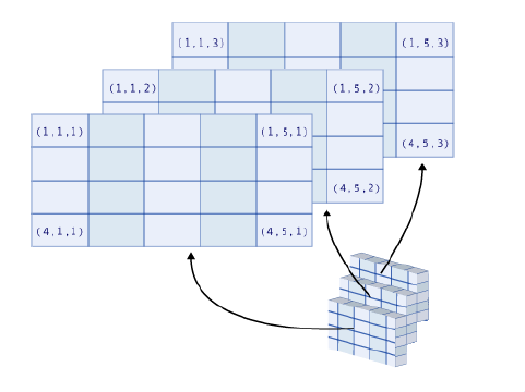
This works under the same rules as it does for vectors, but with multiple dimensions.
(X <- matrix(1:12, nrow=4, ncol=3, byrow=TRUE)) [,1] [,2] [,3]
[1,] 1 2 3
[2,] 4 5 6
[3,] 7 8 9
[4,] 10 11 12X[c(1,4), 2] # Extract the items in the 1st and 4th row and 2nd column[1] 2 11X[c(1,4), -2] # Extract items in the 1st and 4th row but NOT in the 2nd column [,1] [,2]
[1,] 1 3
[2,] 10 12X[c(1,4), -c(2, 3)] # Extract items in the 1st and 4th row but NOT in the 2nd or 3rd columns[1] 1 10We can also omit one of the indices entirely
X[2,][1] 4 5 6As you can see, this extracts the entire second row. Leaving the second dimension empty can be thought of as putting no conditions on it, which means we return everything.
Create a 4 x 5 matrix whose elements are the squares of the first 20 integers (1,2,4,9,16, etc.), populating the matrix one row at a time (starting from the first row). Then, from this matrix, create a sub-matrix by removing the last row and the first column.
(my.X <- matrix((1:20)^2, byrow=TRUE, nrow=4)) [,1] [,2] [,3] [,4] [,5]
[1,] 1 4 9 16 25
[2,] 36 49 64 81 100
[3,] 121 144 169 196 225
[4,] 256 289 324 361 400(sub.X <- my.X[-4,-1]) [,1] [,2] [,3] [,4]
[1,] 4 9 16 25
[2,] 49 64 81 100
[3,] 144 169 196 225Given an operation on two vectors/matrices/arrays of different lengths, R will complete the shortest data structure by repeating its elements from the beginning. We call this behaviour ‘recycling’:
x <- c(1,2,3,4,5,6)
y <- c(1,2,3)
x + y[1] 2 4 6 5 7 9Another example is below, where the vector 1:3 is repeated to fill in a matrix:
matrix(1:3, ncol=3, nrow=4) [,1] [,2] [,3]
[1,] 1 2 3
[2,] 2 3 1
[3,] 3 1 2
[4,] 1 2 3You can merge vectors or matrices together to create a new matrix with functions cbind() and rbind().
(B <- cbind(1:4,5:8)) [,1] [,2]
[1,] 1 5
[2,] 2 6
[3,] 3 7
[4,] 4 8(C <- cbind(B, 9:12)) [,1] [,2] [,3]
[1,] 1 5 9
[2,] 2 6 10
[3,] 3 7 11
[4,] 4 8 12Can you guess what rbind() does?
(A <- matrix(c(2,3,5,4), nrow=2, ncol=2, byrow=T)) [,1] [,2]
[1,] 2 3
[2,] 5 4(B <- matrix(c(1,2,8,7), nrow=2, ncol=2, byrow=F)) [,1] [,2]
[1,] 1 8
[2,] 2 7(I2 <- diag(2)) # identity matrix of size 2x2 [,1] [,2]
[1,] 1 0
[2,] 0 1A+B [,1] [,2]
[1,] 3 11
[2,] 7 11A*B [,1] [,2]
[1,] 2 24
[2,] 10 28A/B [,1] [,2]
[1,] 2.0 0.3750000
[2,] 2.5 0.5714286A%*%I2 [,1] [,2]
[1,] 2 3
[2,] 5 4A%*%B [,1] [,2]
[1,] 8 37
[2,] 13 68t(B) [,1] [,2]
[1,] 1 2
[2,] 8 7Note: the diag() function has other use cases (see R Help or type ?diag if you are curious).
solve(A,b) function can be used to solve \(Ax = b\), for \(x\). Here \(b\) can be a vector or a matrix.solve() is used with only one argument, e.g. solve(A), it will return the inverse of a matrix (if it exists).(A <- matrix(1:4, ncol=2)) [,1] [,2]
[1,] 1 3
[2,] 2 4(x <- solve(A, c(1,1)))[1] -0.5 0.5A%*%x [,1]
[1,] 1
[2,] 1solve(A) %*% A [,1] [,2]
[1,] 1 0
[2,] 0 1The function apply() is often quite handy. It applies a given function to the elements of all rows (MARGIN=1) or all columns (MARGIN=2) of a matrix.
(X <- matrix(c(1:4, 1, 6:8), nrow = 2)) [,1] [,2] [,3] [,4]
[1,] 1 3 1 7
[2,] 2 4 6 8apply(X, MARGIN=1, FUN=median)[1] 2 5apply(X, MARGIN=2, FUN=mean)[1] 1.5 3.5 3.5 7.5Other functions you could use: rowSums(), colSums(), rowMeans(), colMeans().
Given a \(3\times 3\) matrix X
X <- matrix(1:9, nrow = 3)apply to create a vector called row.sums containing the row marginal sums of X (i.e. the sum of elements within each row)(row.sums <- apply(X, 1, sum))[1] 12 15 18col.sums containing the column marginal sums of X(col.sums <- apply(X, 2, sum))[1] 6 15 24sum(row.sums) = sum(col.sums) = sum(X). Make sure you see why that should be the case.(sum(row.sums) == sum(col.sums)) && (sum(X) == sum(row.sums))[1] TRUEDo not confuse ‘data structure’ (vector, matrix, array,…) with ‘data type’ (which we saw in Week 1). A ‘data type’ refers to the type of information (numerical, character, logical, etc.) while a ‘data structure’ refers to how we store (or structure!) the information (in a vector, matrix, data frame, etc.)
This is also an internal (and important) distinction within R. If we want to check the type of information, we use typeof:
typeof(2)[1] "double"typeof("Hello")[1] "character"If we try this on a data structure however, we can see that it actually tells us the type of the objects inside the structure.
typeof(c(1,2,3))[1] "double"typeof(matrix("hi", nrow = 3, ncol = 3))[1] "character"To determine the structure itself, we use class.
class(matrix("hi", nrow = 3, ncol = 3))[1] "matrix" "array" class(data.frame(GENDER=c("F","M","M","F")))[1] "data.frame"class(c(1,2,3))[1] "numeric"class(c("ACTL1101", "ACTL2131", "ACTL3142"))[1] "character"Elements stored in vectors, matrices or arrays need to be of the same type (and R automatically converts them to the same type if they are not).
myVector <- c(1,2,"A", TRUE)
myVector[1] "1" "2" "A" "TRUE"typeof(myVector)[1] "character"Lists can group together, in one structure, data of different types without altering them.
myList <- list(TRUE, my.matrix=matrix(1:4, nrow=2), c(1+2i,3), "R is my friend")
myList[[1]]
[1] TRUE
$my.matrix
[,1] [,2]
[1,] 1 3
[2,] 2 4
[[3]]
[1] 1+2i 3+0i
[[4]]
[1] "R is my friend"The double brackets [[1]] are indicative of a list, and become important to how we extract values in the next slide.
Note that the second item here has a LHS and RHS. When we supply a LHS this “names” the entry in the list, and if we do not, it is left unnamed.
[[]].myList[[3]] # this returns the third item of the list (as "itself")[1] 1+2i 3+0iTo extract several items, use [], but note this will return another list!
myList[1:2] # this returns the 1st and 2nd items of the list, as a list[[1]]
[1] TRUE
$my.matrix
[,1] [,2]
[1,] 1 3
[2,] 2 4We can also use the names of items for extraction.
myList$my.matrix [,1] [,2]
[1,] 1 3
[2,] 2 4Consider ‘myList’ given before as
myList <- list(TRUE, my.matrix=matrix(1:4, nrow=2), c(1+2i,3), "R is my friend")length(myList)[1] 4sapply(myList, typeof) # similar to apply, but works on other data types too my.matrix
"logical" "integer" "complex" "character" class(myList)[1] "list"No. Only the second item is named, as my.matrix.
A data.frame in R is a table where
Data frames are widely used in R
BMI <- data.frame(
Gender=c("M","F","M","F"),
Height=c(1.83,1.78,1.80,1.55),
Weight=c(77,68,66,48),
Names=c("Ben","Katja","Anthony","Jinxia"))
BMI Gender Height Weight Names
1 M 1.83 77 Ben
2 F 1.78 68 Katja
3 M 1.80 66 Anthony
4 F 1.55 48 Jinxiastr(BMI)'data.frame': 4 obs. of 4 variables:
$ Gender: chr "M" "F" "M" "F"
$ Height: num 1.83 1.78 1.8 1.55
$ Weight: num 77 68 66 48
$ Names : chr "Ben" "Katja" "Anthony" "Jinxia"You can access a specific variable using the $ command
BMI$Gender[1] "M" "F" "M" "F"merge() function.X <- data.frame(GENDER=c("F","M","M","F"),
ID=c(123,234,345,456),
NAME=c("Mary","James","James","Olivia"),
Height=c(170,180,185,160))
Y <- data.frame(GENDER=c("M","F","F","M"),
ID=c(345,456,123,234),
NAME=c("James","Olivia","Mary","James"),
Weight=c(80,50,70,60))
X GENDER ID NAME Height
1 F 123 Mary 170
2 M 234 James 180
3 M 345 James 185
4 F 456 Olivia 160Y GENDER ID NAME Weight
1 M 345 James 80
2 F 456 Olivia 50
3 F 123 Mary 70
4 M 234 James 60cbind(X,Y) # Not very useful here GENDER ID NAME Height GENDER ID NAME Weight
1 F 123 Mary 170 M 345 James 80
2 M 234 James 180 F 456 Olivia 50
3 M 345 James 185 F 123 Mary 70
4 F 456 Olivia 160 M 234 James 60merge(X,Y) # This is what we want GENDER ID NAME Height Weight
1 F 123 Mary 170 70
2 F 456 Olivia 160 50
3 M 234 James 180 60
4 M 345 James 185 80Any individual not present in both datasets will be lost.
Z <- data.frame(GENDER=c("M","F","F","F"),
ID=c(345,456,123,999),
NAME=c("James","Olivia","Mary","Jennifer"),
Age=c(21,19,23,99))
Z GENDER ID NAME Age
1 M 345 James 21
2 F 456 Olivia 19
3 F 123 Mary 23
4 F 999 Jennifer 99merge(X,Z) GENDER ID NAME Height Age
1 F 123 Mary 170 23
2 F 456 Olivia 160 19
3 M 345 James 185 21You can use the all.x or all.y arguments to force the inclusion of all the subjects of a dataset.
merge(X,Z, all.x = T) # all subjects of first dataset are kept GENDER ID NAME Height Age
1 F 123 Mary 170 23
2 F 456 Olivia 160 19
3 M 234 James 180 NA
4 M 345 James 185 21merge(X,Z, all.y = T) # all subjects of second dataset are kept GENDER ID NAME Height Age
1 F 123 Mary 170 23
2 F 456 Olivia 160 19
3 F 999 Jennifer NA 99
4 M 345 James 185 21While handling numeric variables is fairly standard in R, we have not examined how to handle categorical variables. For example in the previous data frame,
Z$GENDER # conceptually, this is a categorical variable[1] "M" "F" "F" "F"Z$NAME # this is not, but they are both just treated as strings[1] "James" "Olivia" "Mary" "Jennifer"To tell R to treat the former as a categorical variable, we use factor():
gender_as_factor = factor(Z$GENDER)
levels(gender_as_factor) # this shows you all unique factors[1] "F" "M"While it is difficult to show you how this is helpful just yet, it will become apparent as we do more data manipulation and visualisation.
When necessary, you can also construct ordered categorical variables.
grades = c("P", "HD", "D", "D", "Something Else", "F", "C", "C")
grades_as_factor = factor(grades, levels = c("F", "P", "C", "D", "HD"), ordered = T)
grades_as_factor # note that "Something Else" becomes NA because it isn't specified in levels[1] P HD D D <NA> F C C
Levels: F < P < C < D < HD| Data structure | Instruction in R | Description |
|---|---|---|
| vector | c() | Sequence of elements of the same nature |
| matrix | matrix() | Two-dimensional table of elements of the same nature |
| array | array() | More general than a matrix; table with several dimensions |
| list | list() | Sequence of R structures of any (and possibly different) nature. |
| data frame | data.frame() | Two-dimensional table. The columns can be of different natures, but must have the same length. |
| factor | factor() | Vector of character strings associated with a modality table |
| dates | as.Date() | Vector of dates |
| time series | ts() | Values of a variable observed at several time points |
read.table and read.csv functions (which are widely used to import excel and csv files), but note that other import functions exist, e.g., read.ftable(), scan(), read.delim().read.table() function, it is beneficial to look at an example of raw data.mydata.txt might contain the following:Name,Age,Gender,Income
John,34,M,30
David,36,M,20
Mary,28,F,25
Josephine,32,F,42read.table| Argument name | Description |
|---|---|
| file=path/to/file | Location of the file to be read, including its name with extension (mydata.txt in our example) |
| header=FALSE | Indicates whether the variable names are given on the first line of the file. In the example this is the first line Name,Age,Gender,Income |
| sep=“” | This is the field separator character. Values on each line of the file are separated by this character. (e.g. “” = whitespace, “,” = comma, “\(\backslash\)t” = tabulation). In the example this is a comma. |
| dec=“.” | Decimal mark for numbers (“.” or “,”) |
mydata.txt is in our working directory, we can read the data using the following:data <- read.table(file="mydata.txt", header=TRUE, sep=",").txt file (“mydata.txt”)head(data) or tail(data)head(data) Name Age Gender Income
1 John 34 M 30
2 David 36 M 20
3 Mary 28 F 25
4 Josephine 32 F 42The concept of directories and working directories tends to cause some confusion among students, so here is a brief explanation:
'C:\Users\jose\Desktop\ACTL1101\'R is “working” from.'C:\Users\jose\Desktop\ACTL1101\Assignment'R to look for your data or other files there, you would run setwd('C:/Users/jose/Desktop/ACTL1101/Assignment') (note the change to forward slashes).read.table('mydata.txt', header=T, sep=",") because R is already looking in the right place.As an aside, when you are working from Ed, all requisite files will already be in your working directory (so you do not need to worry about setting the working directory when using Ed).
In the Ed ‘Exercise Space’ for this week we have placed a dataset in the .txt format called danishfire.txt. It contains claim amounts for three different categories of insurance losses, also with the dates at which the losses occurred.
readLines("danishfire.txt", n=5) to visualize the beginning of the data. Note that at this stage you are just looking at the data, you have not imported it.danish_fire.danish_fire by using the head() function.class() and str() to danish_fire. What information does this provide you?mean() and cor().I also encourage you to do this locally (on your own computer)!
# Vizualise data using readLines
readLines("danishfire.txt", n=5)[1] " Positions building contents profits total "
[2] " 01/03/1980 1.09809663 5.856515e-01 0.000000000 1.683748"
[3] " 01/04/1980 1.75695461 3.367496e-01 0.000000000 2.093704"
[4] " 01/05/1980 1.73258126 0.000000e+00 0.000000000 1.732581"
[5] " 01/07/1980 0.00000000 1.305376e+00 0.474377745 1.779754" # import data, note that the header argument is TRUE
danish_fire <- read.table(file="danishfire.txt", header=TRUE, sep="")
head(danish_fire) Positions building contents profits total
1 01/03/1980 1.098097 0.5856515 0.0000000 1.683748
2 01/04/1980 1.756955 0.3367496 0.0000000 2.093704
3 01/05/1980 1.732581 0.0000000 0.0000000 1.732581
4 01/07/1980 0.000000 1.3053760 0.4743777 1.779754
5 01/07/1980 1.244510 3.3674960 0.0000000 4.612006
6 01/10/1980 4.452040 4.2732340 0.0000000 8.725274class(danish_fire)[1] "data.frame"str(danish_fire)'data.frame': 2167 obs. of 5 variables:
$ Positions: chr "01/03/1980" "01/04/1980" "01/05/1980" "01/07/1980" ...
$ building : num 1.1 1.76 1.73 0 1.24 ...
$ contents : num 0.586 0.337 0 1.305 3.367 ...
$ profits : num 0 0 0 0.474 0 ...
$ total : num 1.68 2.09 1.73 1.78 4.61 ...# some numerical analysis
mean(danish_fire$building)[1] 1.824408cor(danish_fire$building, danish_fire$contents)[1] 0.3271123Note that function readLines() is useful as it allows you to visualize the beginning of the data file before you import the data, so you know the structure of the data and can determine the arguments of the function read.table().
csv), most arguments of the function read.table() are fixed.read.table() with several arguments filled with pre-determined values, e.g.,
read.csv(): .csv format (csv stands for comma separated values)movies.data <- read.csv("Movies.csv")
head(movies.data) Movie.ID Movie.Title Release.Year Runtime
1 1 Harry Potter and the Philosopher's Stone 2001 152
2 2 Harry Potter and the Chamber of Secrets 2002 161
3 3 Harry Potter and the Prisoner of Azkaban 2004 142
4 4 Harry Potter and the Goblet of Fire 2005 157
5 5 Harry Potter and the Order of the Phoenix 2007 138
6 6 Harry Potter and the Half-Blood Prince 2009 153
Budget Box.Office
1 $125,000,000 $1,002,000,000
2 $100,000,000 $880,300,000
3 $130,000,000 $796,700,000
4 $150,000,000 $896,400,000
5 $150,000,000 $942,000,000
6 $250,000,000 $943,200,000 read.csv() will do the trick.read.table() is important.Create a data frame that contains only the first 50 rows of danish_fire, and then export this new data set to a folder on your computer.
# Create the new data set
danish.50.only <- danish_fire[1:50,]
# Exporting data to a text file
write.table(danish.50.only, file = "myfile.txt", sep = "\t")
# Exporting data to a csv file
write.csv(danish.50.only, file = "myfile.csv")Note that the commands above save your data into the working directory.
If you are using R on your computer (not in Ed!), you can specify a different path if you wish, by using file = "path/to/data/myfile.txt".
Generate a random vector of 1000 standard normal observations. Then,
Give the R instruction which gives the following output:
> A
     [,1] [,2] [,3]
[1,]    1    5    9
[2,]    2    6   10
[3,]    3    7   11
[4,] 4 8 12Assuming that A was created as above, predict the outputs of the following instructions:
A[3,]A[2,2:3]Given two matrices \(A\) and \(B\), where: \[ A = \begin{bmatrix} 1 & 2 \\ 3 & 4 \end{bmatrix} \quad \text{ and } \quad B = \begin{bmatrix} 5 & 6 \\ 7 & 8 \end{bmatrix} \] Find the following:
Give the instruction to merge these two tables:
> X
  Gender Weight Names
1      M     80  Jack
2      F     60 Julia
> Y
   Eyes Height Names
1  Blue    180  Jack
2 Green 160 JuliaName the main data structures available in R.
What is the main advantage of the “list” data structure?
What is the purpose of the following R functions:
read.table()read.csv()write.table()write.csv()Import the file called Movie.csv into your working directory (and store it as a data frame, with a name of your choice). Note you can find this file under Ed Resources. Then, find the average Runtime of all Harry Potter movies. What happens if you try to find their average Box.Office?
By using ‘logical masks’: X[mask]
Mat <- matrix(1:12,nrow=4,byrow=TRUE)
MatLogical <- matrix(c(TRUE,FALSE),nrow=4,ncol=3)
Mat
[,1] [,2] [,3]
[1,] 1 2 3
[2,] 4 5 6
[3,] 7 8 9
[4,] 10 11 12MatLogical [,1] [,2] [,3]
[1,] TRUE TRUE TRUE
[2,] FALSE FALSE FALSE
[3,] TRUE TRUE TRUE
[4,] FALSE FALSE FALSEMat[MatLogical][1] 1 7 2 8 3 9m <- matrix(c(1,2,3,1,2,3,2,1,3),3,3)
m [,1] [,2] [,3]
[1,] 1 1 2
[2,] 2 2 1
[3,] 3 3 3which(m == 1) [1] 1 4 8The outputs of 1, 4, and 8 can be found by counting from top to bottom and then left to right across the 2 dimensions of the matrix.
However, we can get a more meaningful output
which(m == 1,arr.ind=TRUE) row col
[1,] 1 1
[2,] 1 2
[3,] 2 3# this gives the indices (row and column) of all elements = 1