Week 8: Introduction to ggplot2

Learning outcomes

By the end of this topic, students should be able to

draw and edit curves and plots with ggplot2;
present and summarise statistical data with visualisation tools in gglot2;
know where to look for to further learn R

ggplot2 basics

ggplot2 - Introduction

ggplot2 is a package in R that offers a wide range of visualisation tools.
The language of ggplot2 is always the same:
- You add ‘building blocks’ of visualisation (data, statistical transformations, coordinate system, labels,…) one at a time using ‘+’
It is a natural way of creating plots.
It allows advanced visualisation in a simple way.

Reference

ggplot2 - Introduction

The basic function is ggplot()

ggplot(raw_data)

An empty plot is created.
A dataset is supplied, but with no further instruction on how the data should be presented, hence nothing is displayed.
Importantly, the data set supplied (here ‘raw_data’) must be a data frame.

ggplot2 - Geoms

A geom is a function that returns a layer of visualisation.
There are many different geom in ggplot2, to visualise data in different ways:
- geom_point - scatter graph
- geom_line - line graph
- geom_boxplot - box plot
- geom_histogram - histogram
- geom_abline - adds a straight line, specified by intercept and slope
- geom_smooth - adds a line/curve of best fit
- etc.

ggplot2 - Geoms

Now, let’s use geom_point to create a scatter graph.

ggplot(raw_data)+geom_point(aes(x = height, y = weight))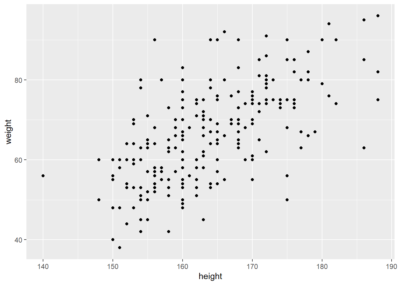

Note the plus ‘+’ sign after the ggplot() function.
aes() stands for ‘aesthetic’. Different geoms have different required aesthetics but these are generally features of the visualisation that should be determined by the data.
For a scatter plot we need the x and y coordinates to be determined by the data, hence we use aes(x = height, y = weight)
Another subtle point is that geom_point is actually “inheriting” the data argument raw_data from ggplot(raw_data). It would be equally valid to write:

ggplot() + geom_point(raw_data, aes(x = height, y = weight))

We will see more on this and how it can be used later.

Exercise

Using sample_data.csv, create a boxplot for the variable weight by the variable meat.

Solution

raw_data<-read.csv("sample_data.csv",header=TRUE)
ggplot(raw_data)+geom_boxplot(aes(meat,weight))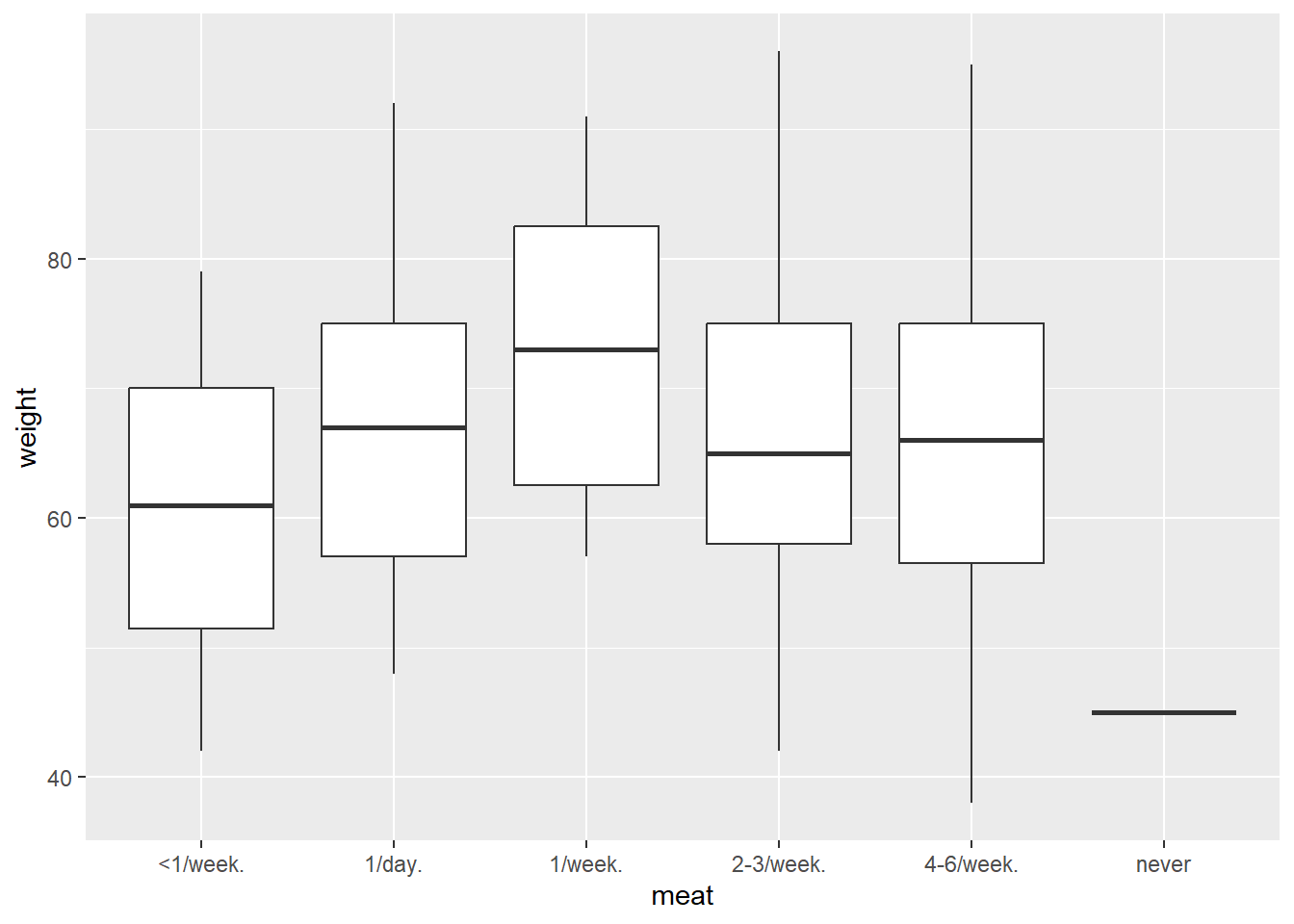

ggplot2 - Geoms

Many ‘geoms’ can be combined

ggplot(raw_data)+ 
  geom_point(aes(height, weight))+ # draw points 
  geom_abline(intercept = -70, slope = 0.8) # add line (note this is not the best fit, just a line with arbitrary values)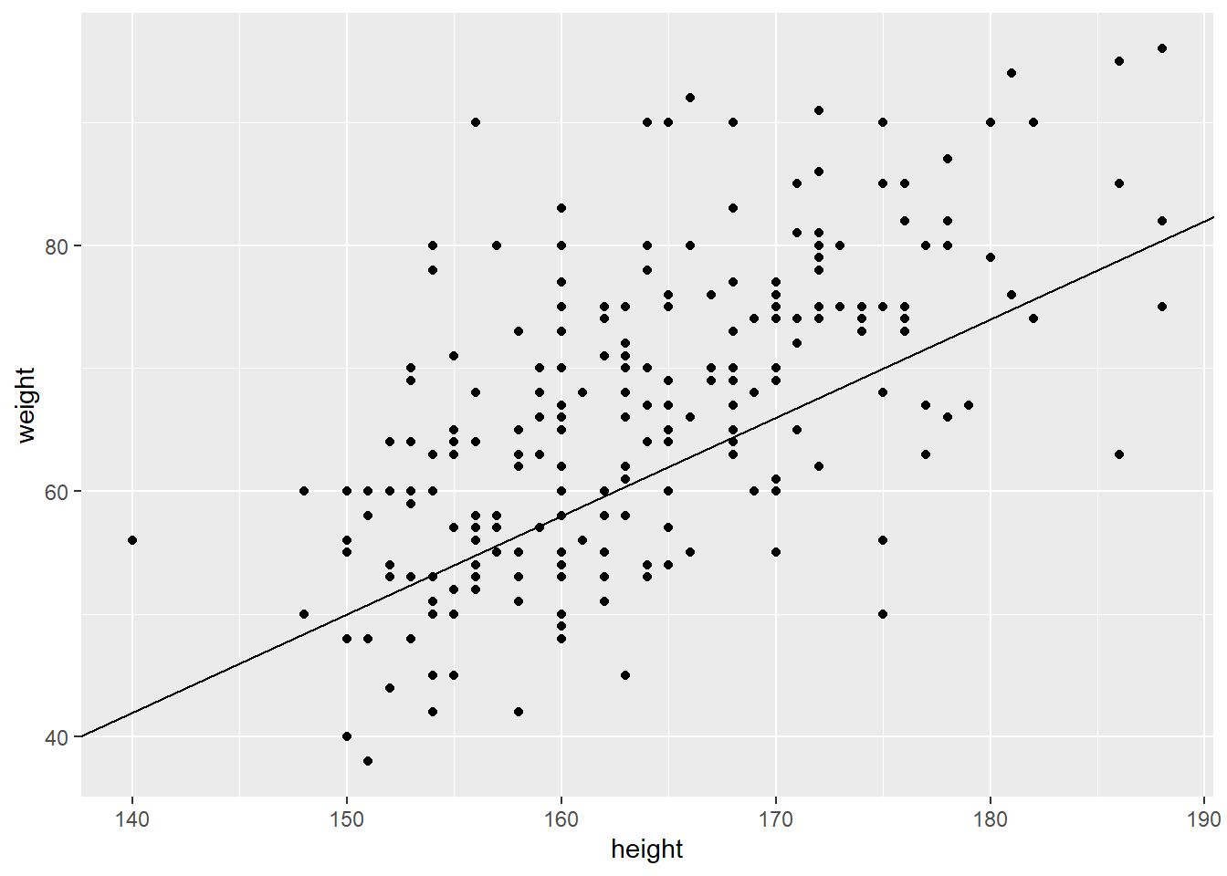

ggplot2 - Geoms

One can also create the line with the geom_smooth() function.

ggplot(raw_data, aes(height, weight))+
  geom_point()+
  geom_smooth(method = "lm", se = TRUE)+ # this adds the best linear fit to the data
  labs(x = "Height", y = "Weight",
    title ="Line Chart of Height against Weight",
    subtitle = "A simple illustration",
    caption = "This graph shows the relationship between height and weight")
## `geom_smooth()` using formula = 'y ~ x'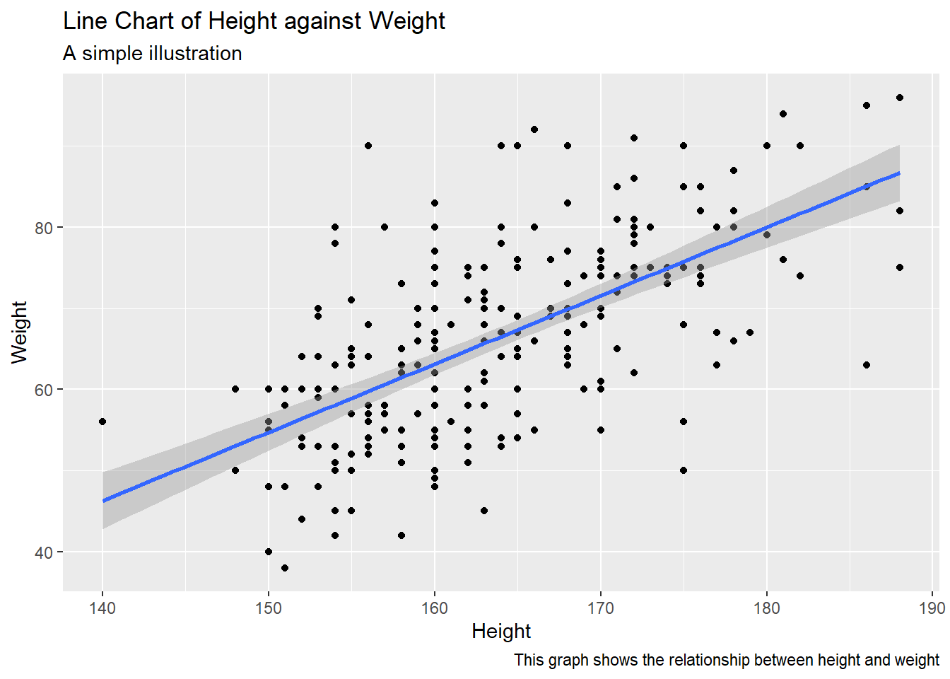

Notes:

The option se=TRUE displays the confidence interval on the fitted line (stay tuned for the maths of this in ACTL2131, a second year course)
This further shows how the inheritance works in ggplot. In this case, raw_data and aes(height, weight) were inherited by both geom_point and geom_smooth, and in fact any other further geoms would also inherit them. This significantly reduces repetition when it is appropriate.
labs is used to customise any fixed label, i.e. x and y axes, the main title, legend titles, etc.

Exercise

Use the iris dataset. Create a histogram for the variable Petal.Length. Add appropriate labels (x-axis, y-axis) and a title to the plot.

Solution

Note that one should adjust the binwidth.

ggplot(iris)+
  geom_histogram(aes(Petal.Length), binwidth=0.5)+
  labs(x = "Weight", y = "Number of observations",
 title ="Histogram for the variable Petal.Length")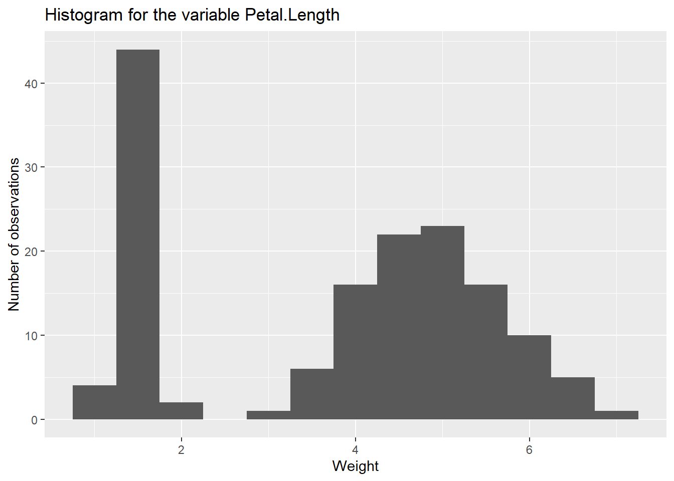

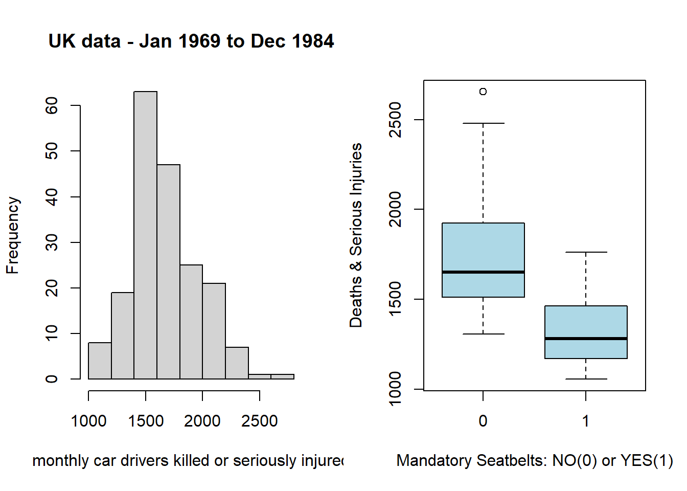
Exercise

Use the Seatbelts dataset to recreate the following two graphs from last week’s lab in ggplot: a histogram of the drivers column, and a boxplot of drivers by law. Do not worry about the colouring or theme for now, we will discuss that later.

Solution

data <- as.data.frame(Seatbelts)
ggplot(data) +
  geom_histogram(aes(drivers), bins = 10) +
  labs(x = "monthly car drivers killed or seriously injured", 
       title = "Histogram of  UK - Jan 1969 to Dec 1984")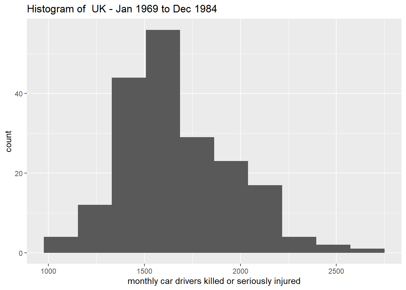

Solution

# convert variable 'law' in a factor
data$law <- factor(data$law,  labels = c("0", "1"))
ggplot(data) +
  geom_boxplot(aes(x = law, y = drivers)) +
  labs(x = "Mandatory Seatbelts: NO(0) or YES(1)", 
       y = "Deaths & Serious Injuries")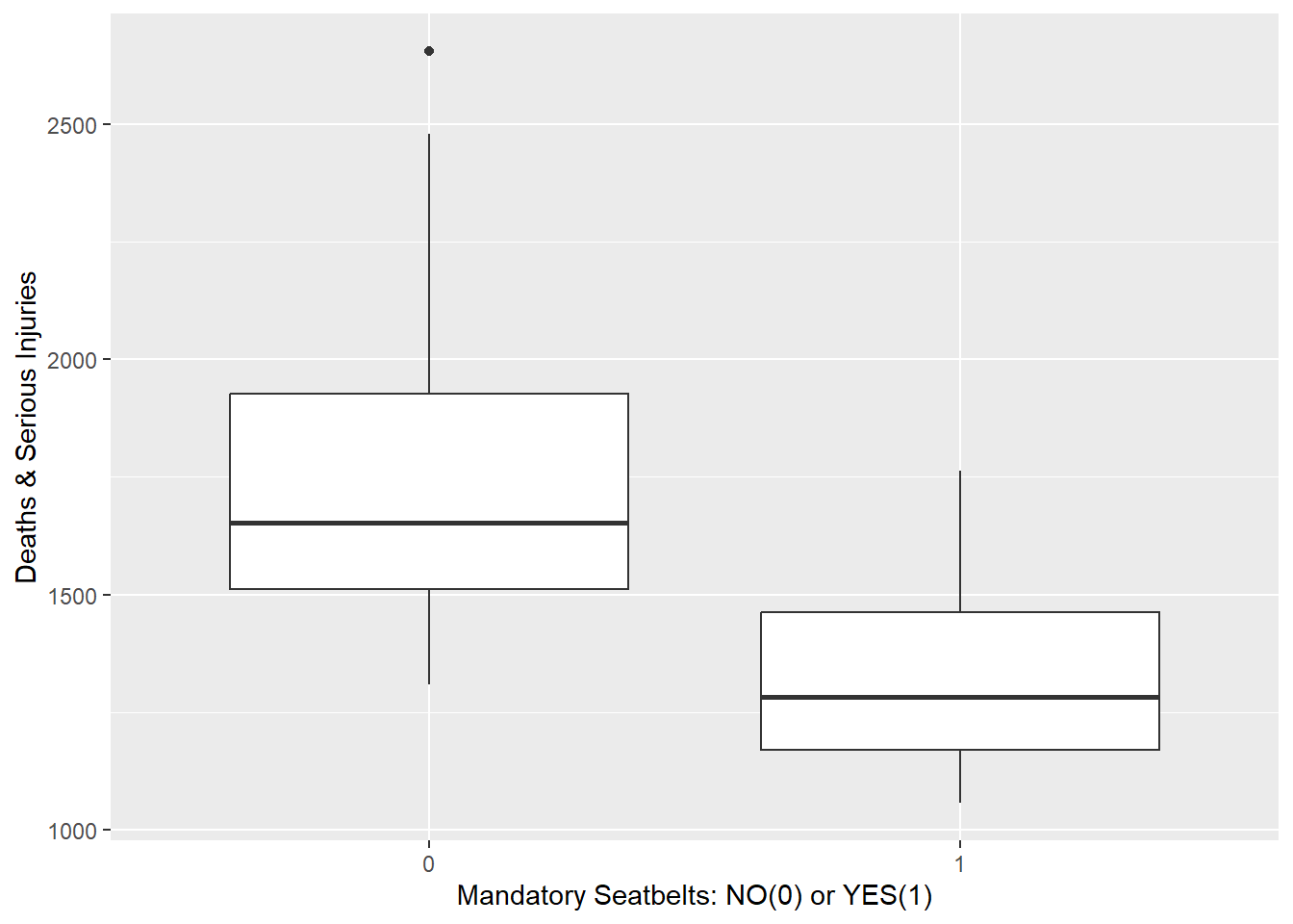

ggplot2 - Stats

Another type of visual layer you can add with ggplot2 is a stat. For example, you can use the stat_ecdf() to visualise the empirical distribution function of a continuous variable.

ggplot(raw_data, aes(height)) +
  stat_ecdf() + labs(y = 'Empirical CDF')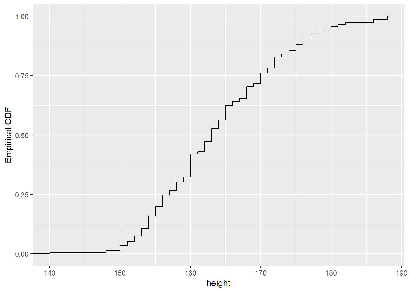

In fact, both a stat and a geom are required for any visual layer!
But when you use for example geom_point, it actually is by default selecting the geom point and the stat identity
Similarly, stat_ecdf is defaulting to the stat ecdf and the geom step
If this is confusing you do not have to worry about it too much it’s just some extra knowledge. For those that are interested you can read more here

ggplot2 - Stats

stats are used when ggplot2 needs to calculate a new variable to plot
stat_function can be used to directly plot a function, for example a normal distribution density function as below

ggplot(data = data.frame(x = c(-3, 3)), aes(x)) +
  stat_function(fun = dnorm, n = 100, args = list(mean = 0, sd = 1))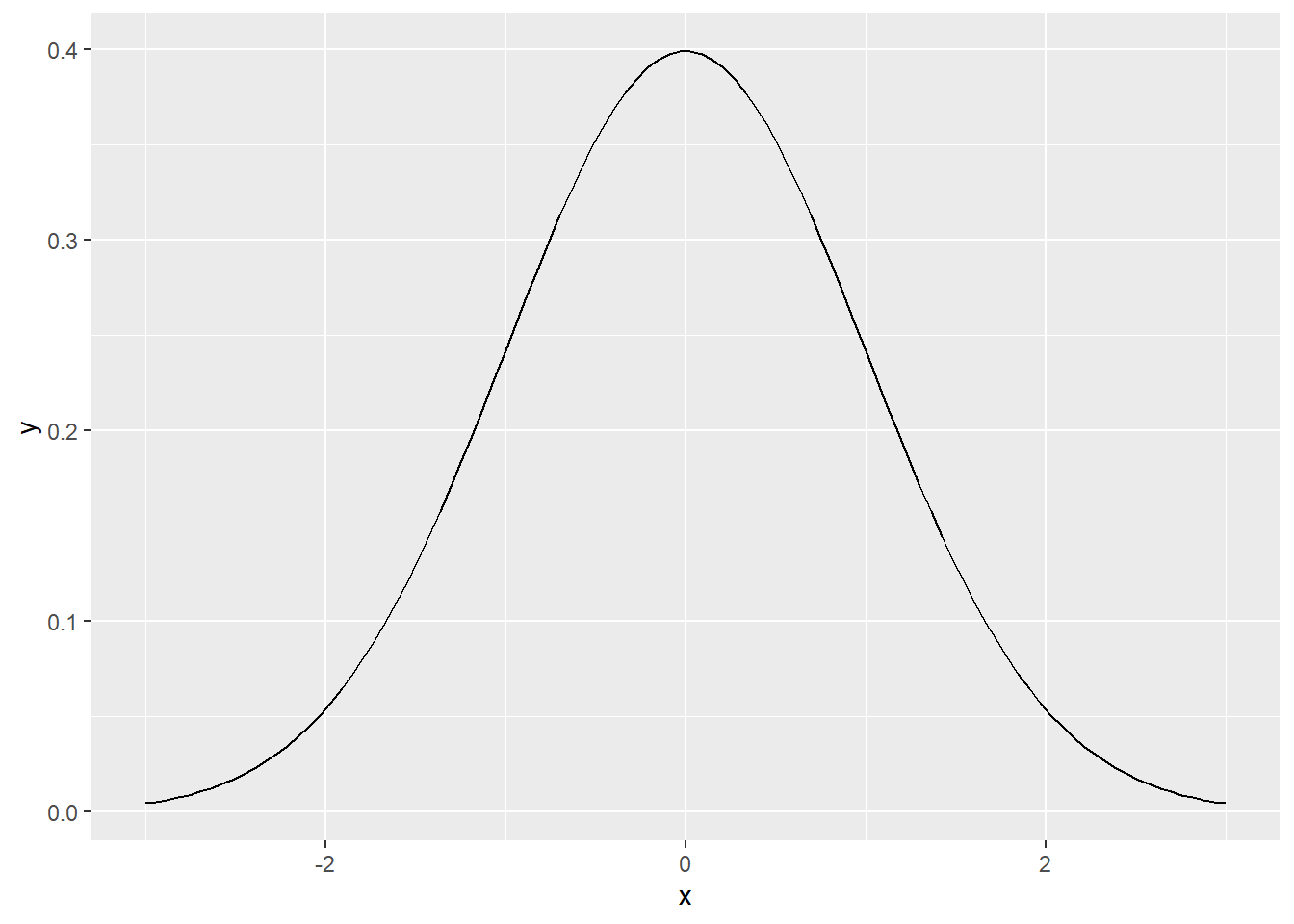

Exercise

Use stat_function to plot:

A lognormal(0,1) cumulative distribution function on the interval(0,10)
The function:

\[y=x^2+2x+4-e^{1-x^2}\] on the interval(-1,1)

Solution

ggplot(data = data.frame(x = c(0, 10)), aes(x)) +
  stat_function(fun = plnorm, n = 100, args = list(mean = 0, sd = 1))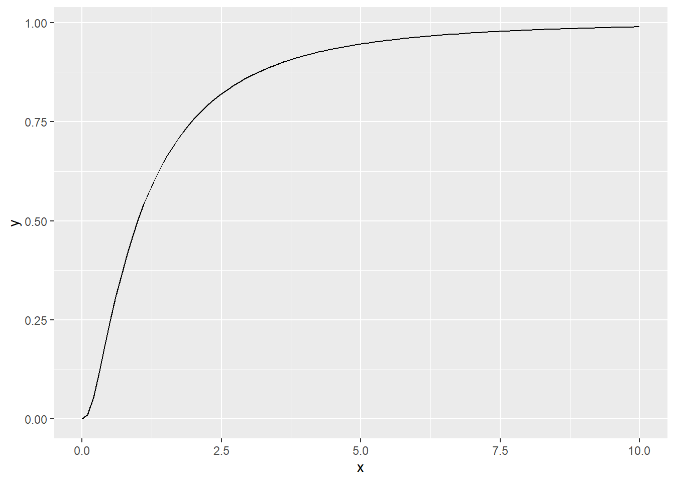

Solution

f = function(x) {
  return(x^2+2*x+4-exp(1-x^2))
}
ggplot(data = data.frame(x = c(-1, 1)), aes(x)) +
  stat_function(fun = f, n = 100)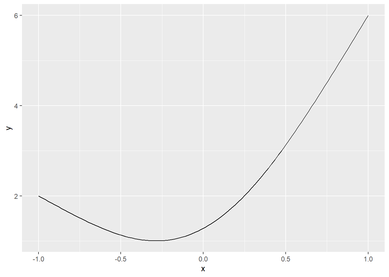

ggplot2 - Themes

ggplot2 offers a range of built-in themes to improve the presentation of your plots, by changing their overall aspect

ggplot(raw_data,aes(height))+stat_ecdf()+theme_bw()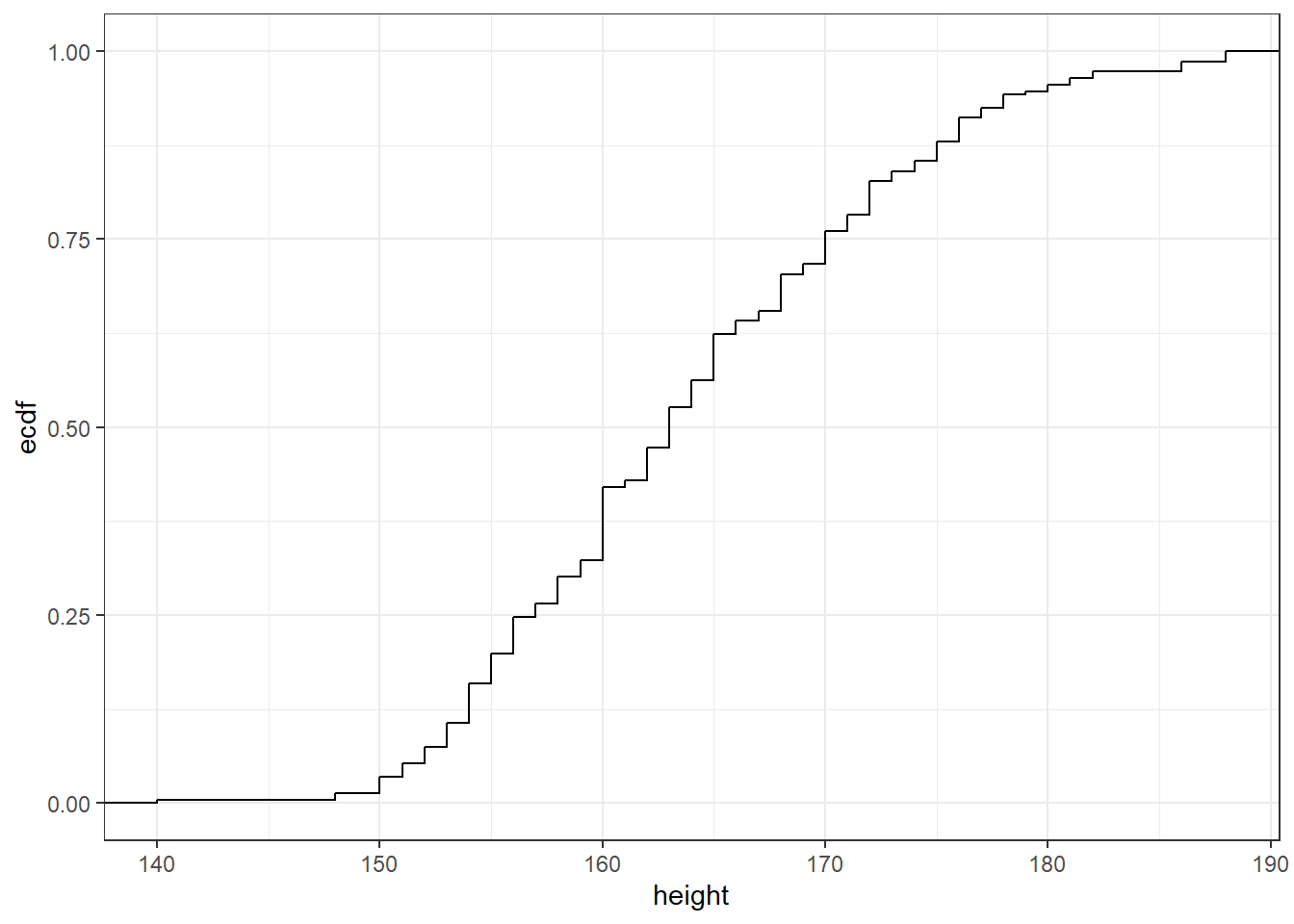

ggplot(raw_data,aes(height))+stat_ecdf()+theme_classic()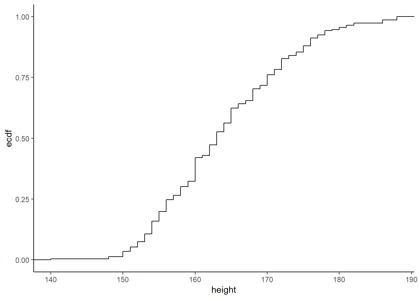

ggplot(raw_data,aes(height))+stat_ecdf()+theme_dark()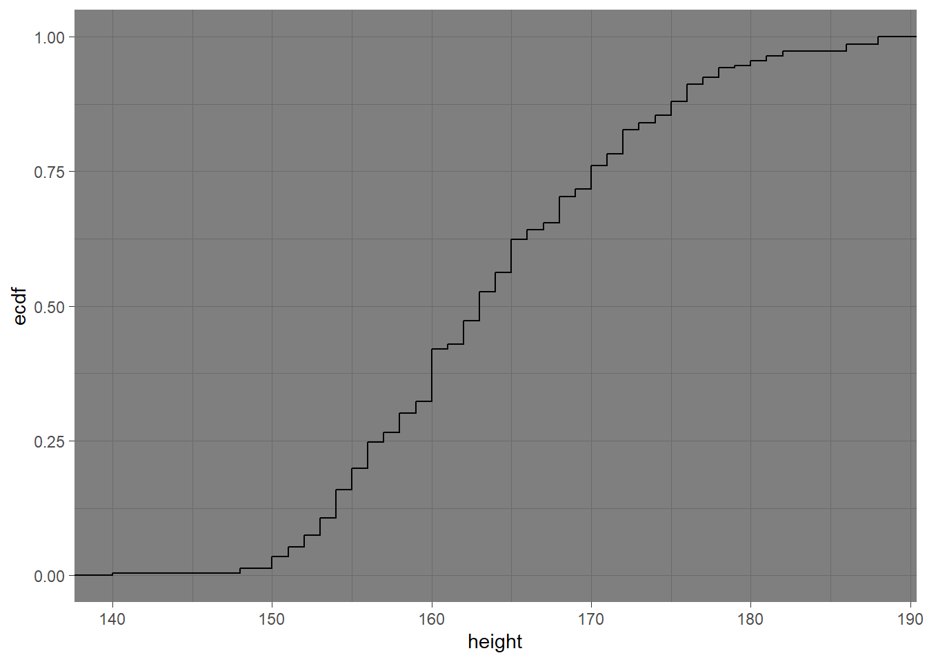

Additional Reference

ggplot2 - Other Aesthetics

An important part of visualisation is categorising different observations, for example by colour, shape, size or transparency. ggplot provides convenient syntax for this.

For example, say we want to produce a plot like this:

ggplot2 - Other Aesthetics

We start with a plain ggplot. Dataset midwest (also from ggplot2 package) contains demographic information of midwest counties (such as total population, area, state, population density, etc) in the USA.

ggplot(midwest, aes(x=area, y=poptotal)) + 
  geom_point() +  
  xlim(c(0, 0.1)) +  # plot inside a range that suit us
  ylim(c(0, 500000)) +
  theme(text = element_text(size=20)) #make axis bigger
## Warning: Removed 15 rows containing missing values or values outside the scale range
## (`geom_point()`).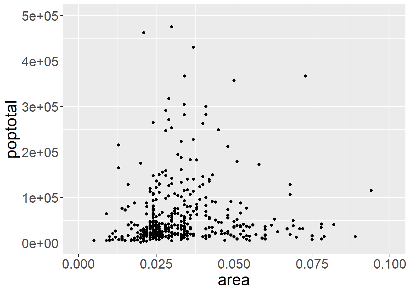

As mentioned before, providing extra arguments to aes tells ggplot to alter how each data point is visualised based on the value of that data point. Based on this we can also supply arguments like color and size:

The color can be used to categorise observations, different ‘states’ in the current example
The sizes can be used to indicate numerical values, different ‘population densities’ in the current example

ggplot(midwest, aes(x=area, y=poptotal)) + 
  geom_point(aes(color=state, size=popdensity)) +  
  xlim(c(0, 0.1)) +  # plot inside a range that suit us
  ylim(c(0, 500000)) +
  theme(text = element_text(size=20)) #make axis bigger
## Warning: Removed 15 rows containing missing values or values outside the scale range
## (`geom_point()`).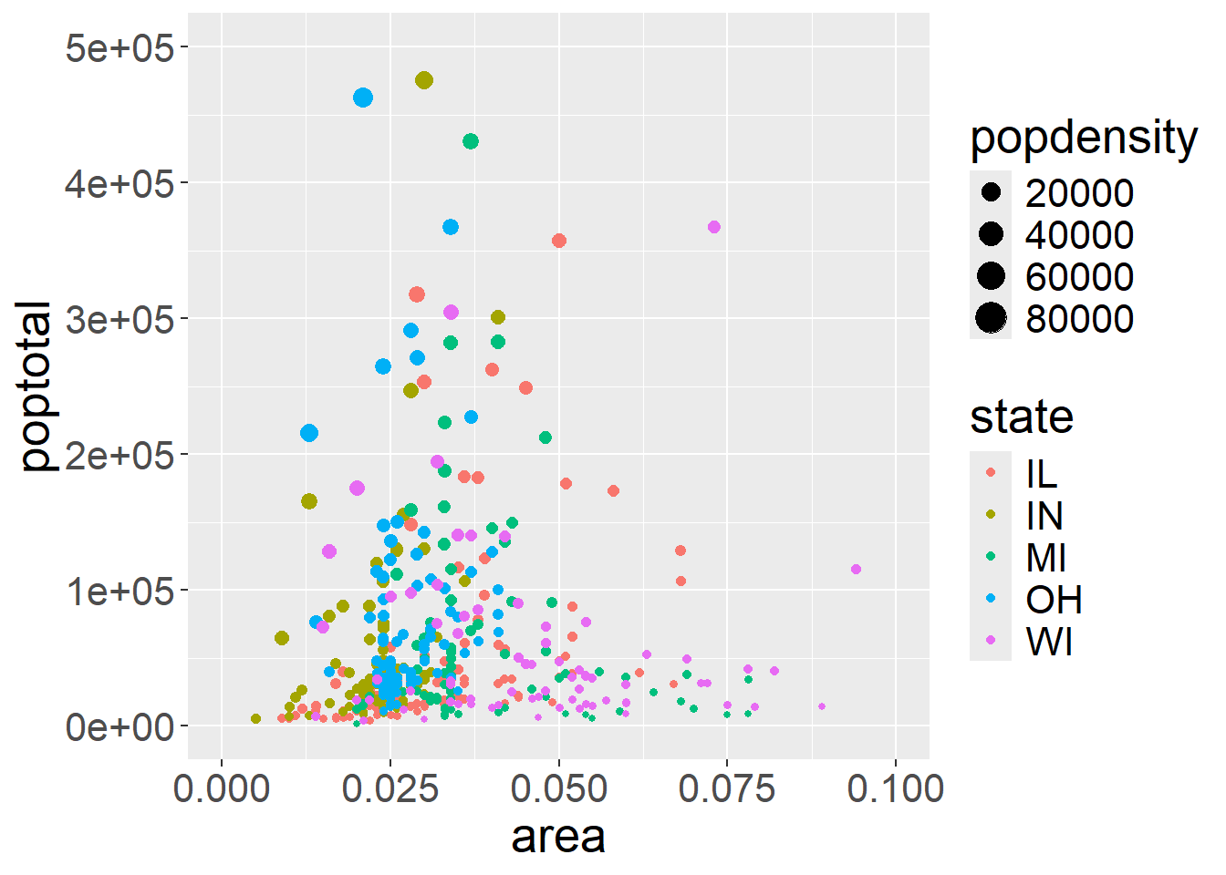

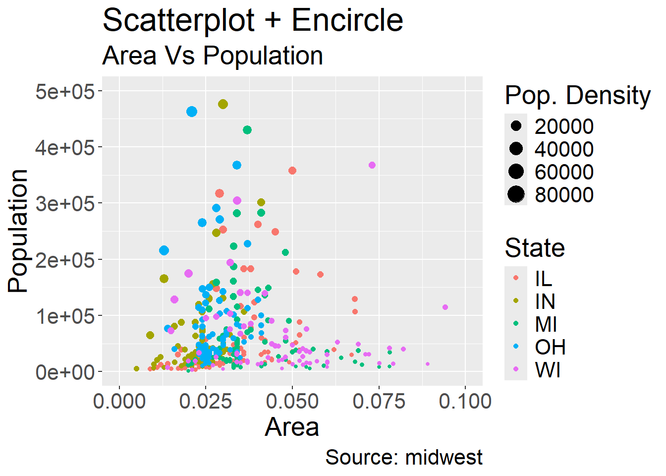
Reference

ggplot2 - Other Aesthetics

Conveniently, this also creates a legend for us by default however the naming is quite poor. We can fix this yet again using the labs argument:

ggplot(midwest, aes(x=area, y=poptotal)) + 
  geom_point(aes(col=state, size=popdensity)) +   # draw points
  xlim(c(0, 0.1)) + 
  ylim(c(0, 500000)) +   # draw smoothing line
  labs(subtitle="Area Vs Population", 
       y="Population", 
       x="Area", 
       title="Scatterplot + Encircle", 
       caption="Source: midwest",
       color="State",
       size="Pop. Density") +
    theme(text = element_text(size=20)) #make axis/labels bigger
## Warning: Removed 15 rows containing missing values or values outside the scale range
## (`geom_point()`).

There are also other aesthetics that are often used for similar purposes:

alpha indicates numerical values as well by adjusting the transparency
shape indicates categorical values by adjusting the shape of the points
fill works similarly to colour but for other geoms. For example, in a bar plot, fill is the colour of the bar, while colour is the border colour

More Advanced Examples

Advanced Example 1

In addition to a simple scatter plot, it may also be useful to know the number of observations at each point, and the marginal distributions:

## `geom_smooth()` using formula = 'y ~ x'
## `geom_smooth()` using formula = 'y ~ x'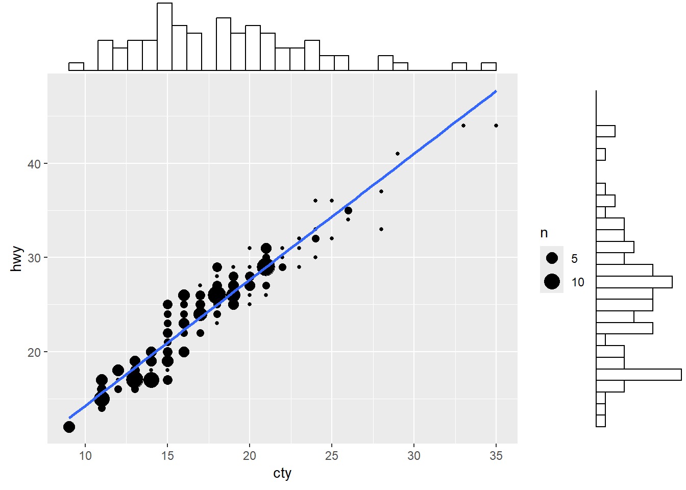

Advanced Example 1

We start from a standard scatter plot of variable hwy vs cty (highway and city ‘miles per gallon’, for various car models) from data set mpg (included in the ggplot2 package).

ggplot(mpg, aes(cty, hwy)) + 
  geom_point()+ 
  geom_smooth(method="lm", se=F) + 
  theme_bw()
## `geom_smooth()` using formula = 'y ~ x'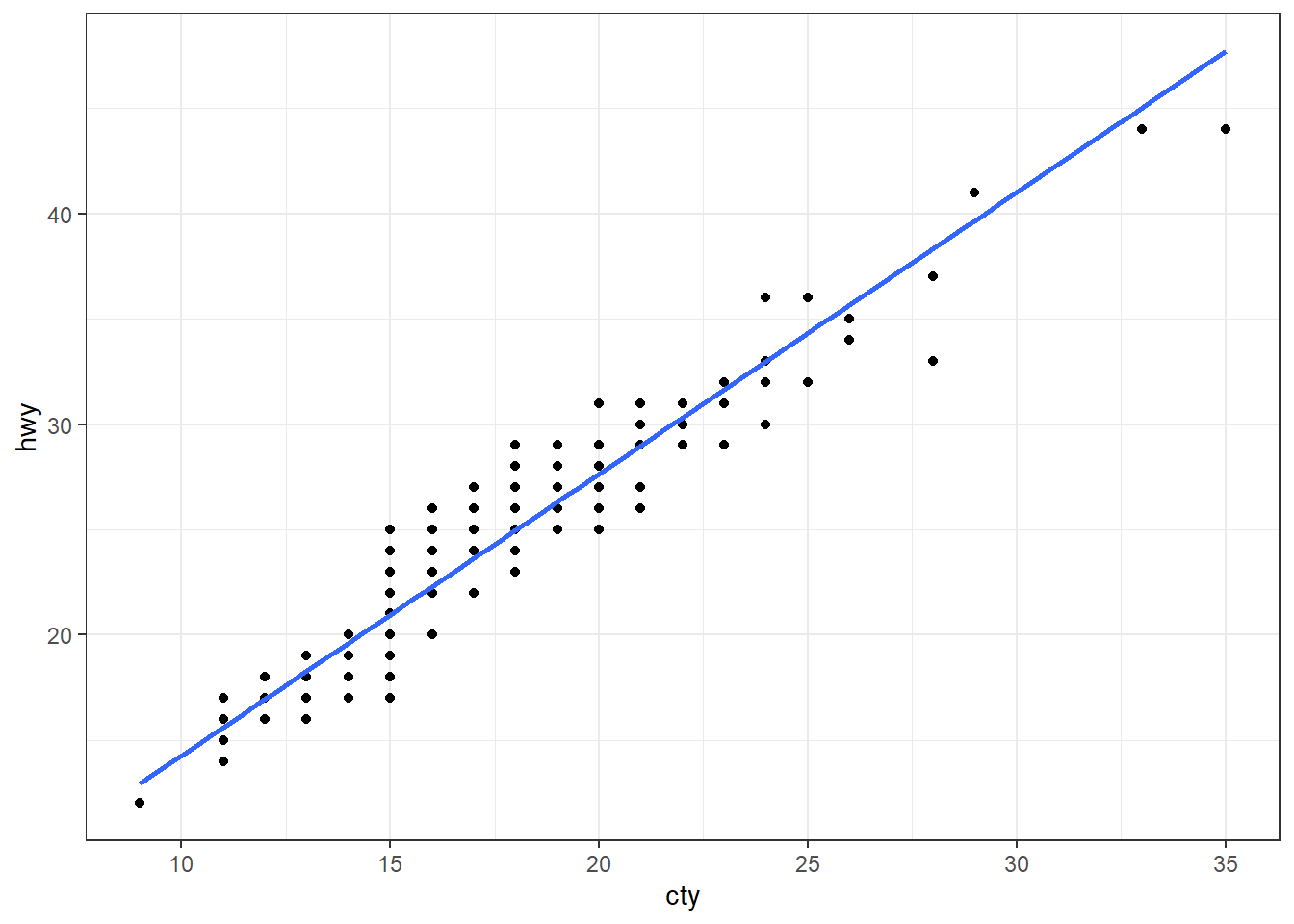

Have a look at the data set. Are cty and hwy truly continuous variables? What problem does this create?

Reference

Advanced Example 1

head(mpg, 10)
## # A tibble: 10 × 11
##    manufacturer model      displ  year   cyl trans drv     cty   hwy fl    class
##    <chr>        <chr>      <dbl> <int> <int> <chr> <chr> <int> <int> <chr> <chr>
##  1 audi         a4           1.8  1999     4 auto… f        18    29 p     comp…
##  2 audi         a4           1.8  1999     4 manu… f        21    29 p     comp…
##  3 audi         a4           2    2008     4 manu… f        20    31 p     comp…
##  4 audi         a4           2    2008     4 auto… f        21    30 p     comp…
##  5 audi         a4           2.8  1999     6 auto… f        16    26 p     comp…
##  6 audi         a4           2.8  1999     6 manu… f        18    26 p     comp…
##  7 audi         a4           3.1  2008     6 auto… f        18    27 p     comp…
##  8 audi         a4 quattro   1.8  1999     4 manu… 4        18    26 p     comp…
##  9 audi         a4 quattro   1.8  1999     4 auto… 4        16    25 p     comp…
## 10 audi         a4 quattro   2    2008     4 manu… 4        20    28 p     comp…

Many values of cty and hwy are repeated, hence many points overlap
This means the previous plot does not show all points
We can solve this by showing the number of observations at each spot, using the size of the dot as an indicator.
This is simply done by replacing geom_point() with geom_count().

ggplot(mpg, aes(cty, hwy)) + 
  geom_count() + 
  geom_smooth(method="lm", se=F)  + 
  theme_bw()
## `geom_smooth()` using formula = 'y ~ x'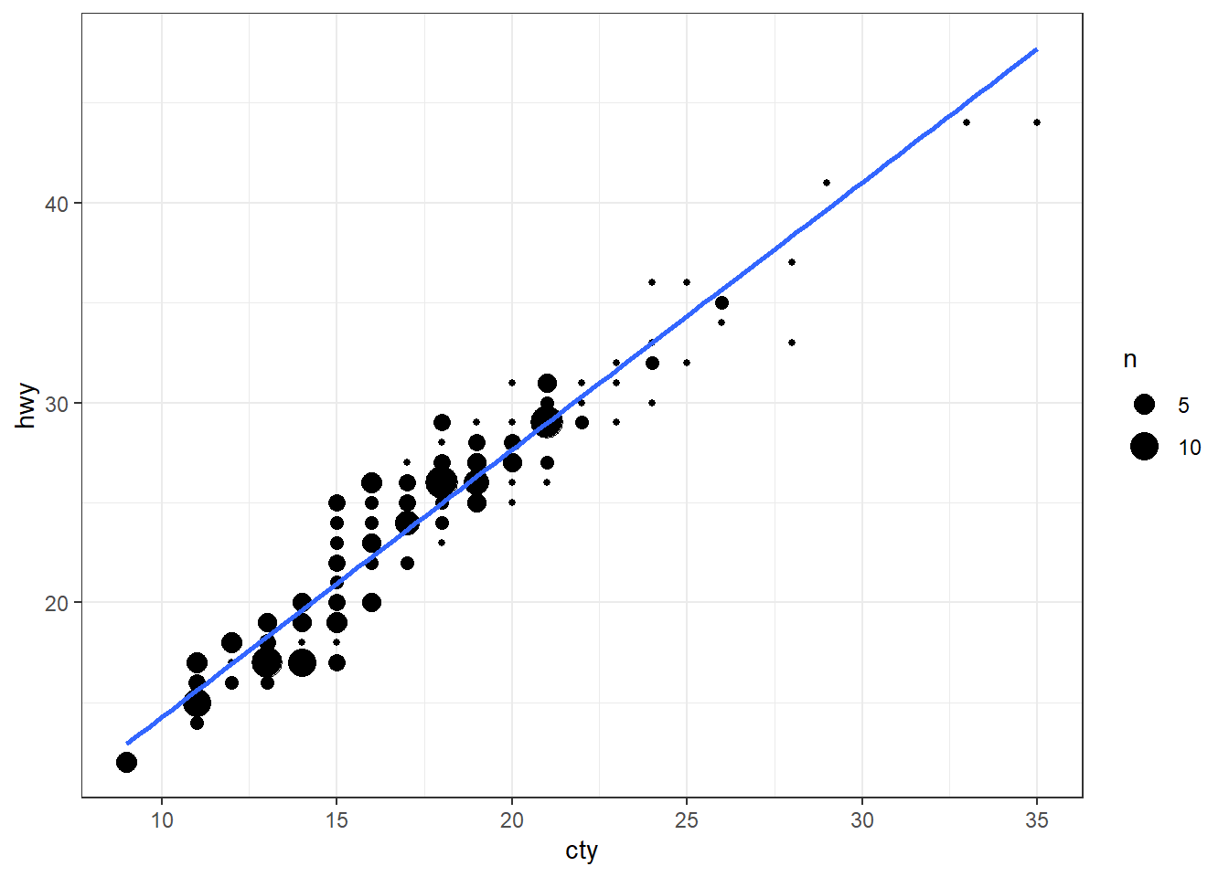

Reference

Advanced Example 1

A scatter plot illustrates how two variables are related, but it could be useful to have a quick idea of their individual (marginal) distributions as well.

The ggMarginal() function from the ggExtra package allows to visualise marginal distributions on top of a scatter plot. Below we add a histogram of marginal distributions on top of the scatter plot.

g <- ggplot(mpg, aes(cty, hwy)) + 
  geom_count() + 
  geom_smooth(method="lm", se=F) +
  theme_set(theme_bw())
  
ggMarginal(g, type = "histogram", fill="transparent")
## `geom_smooth()` using formula = 'y ~ x'
## `geom_smooth()` using formula = 'y ~ x'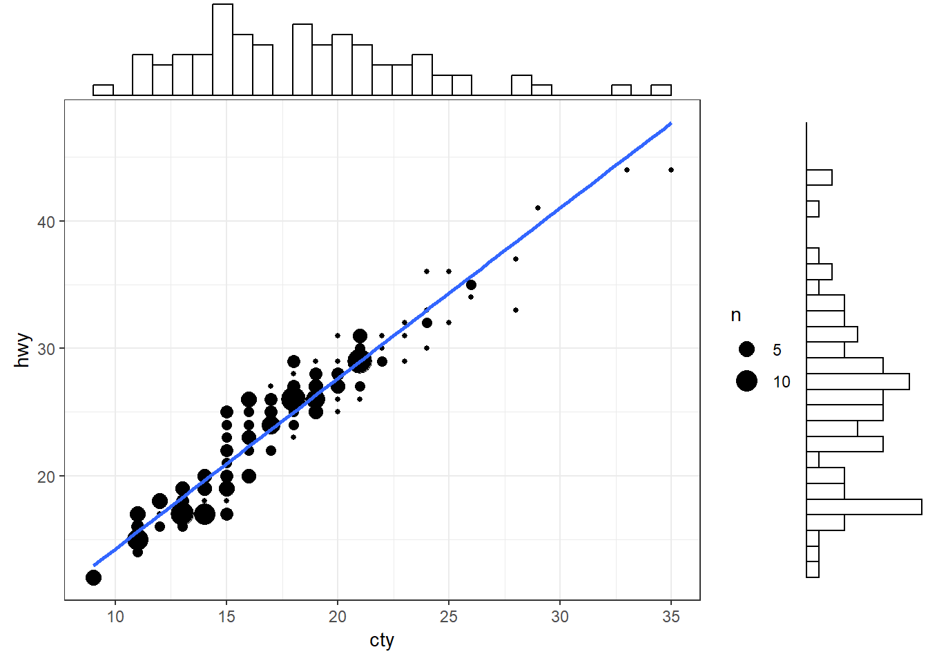

One can also add an (estimated) smooth density instead of a histogram for each margin.

g <- ggplot(mpg, aes(cty, hwy)) + 
  geom_count() + 
  geom_smooth(method="lm", se=F)+
  theme_set(theme_bw()) 

ggMarginal(g, type = "density", fill="transparent")
## `geom_smooth()` using formula = 'y ~ x'
## `geom_smooth()` using formula = 'y ~ x'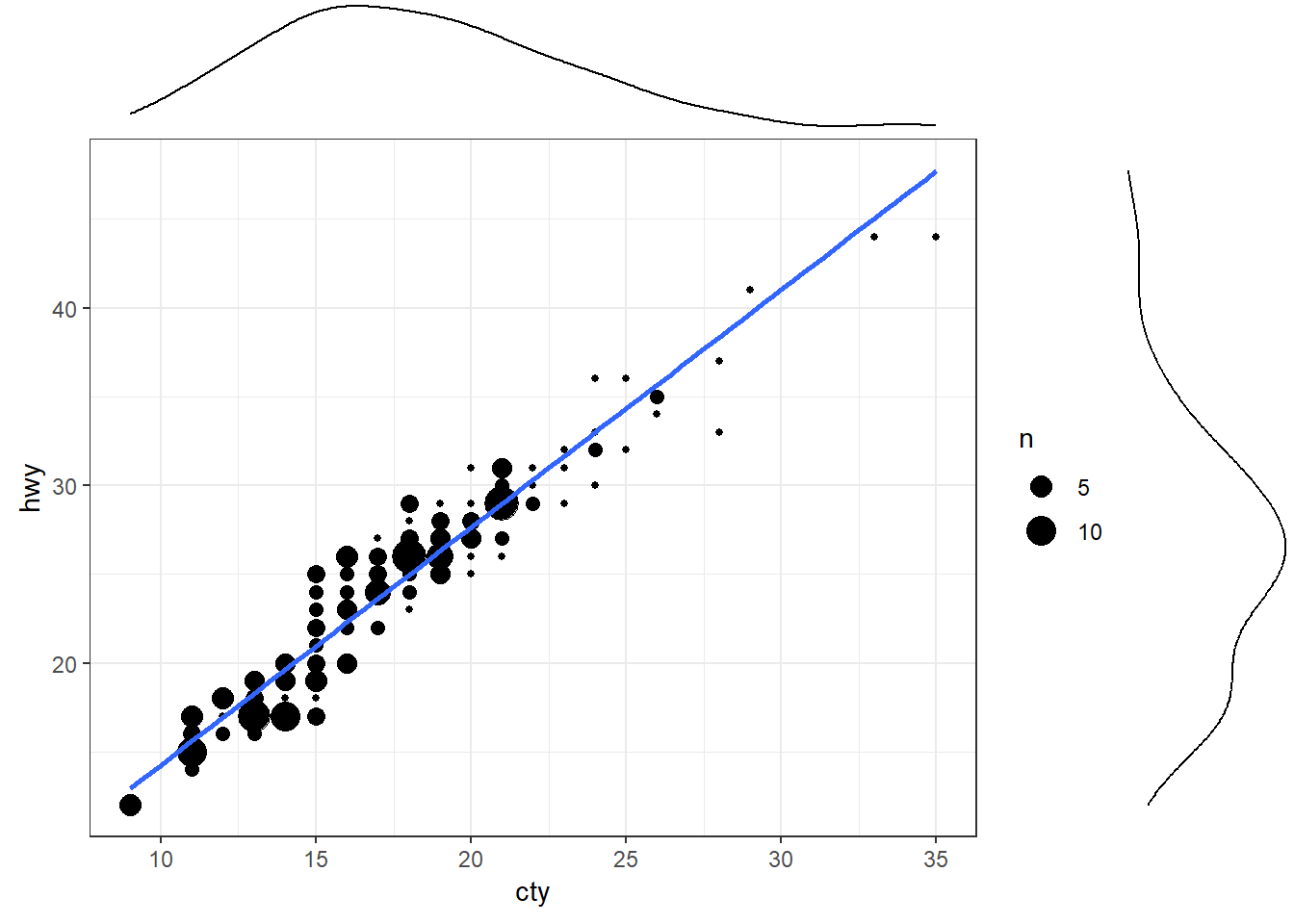

Reference

Advanced Example 2

Coming back to the example we gave for “Other Aesthetics”, sometimes it is also useful to be able to encircle or highlight some data:

Advanced Example 2

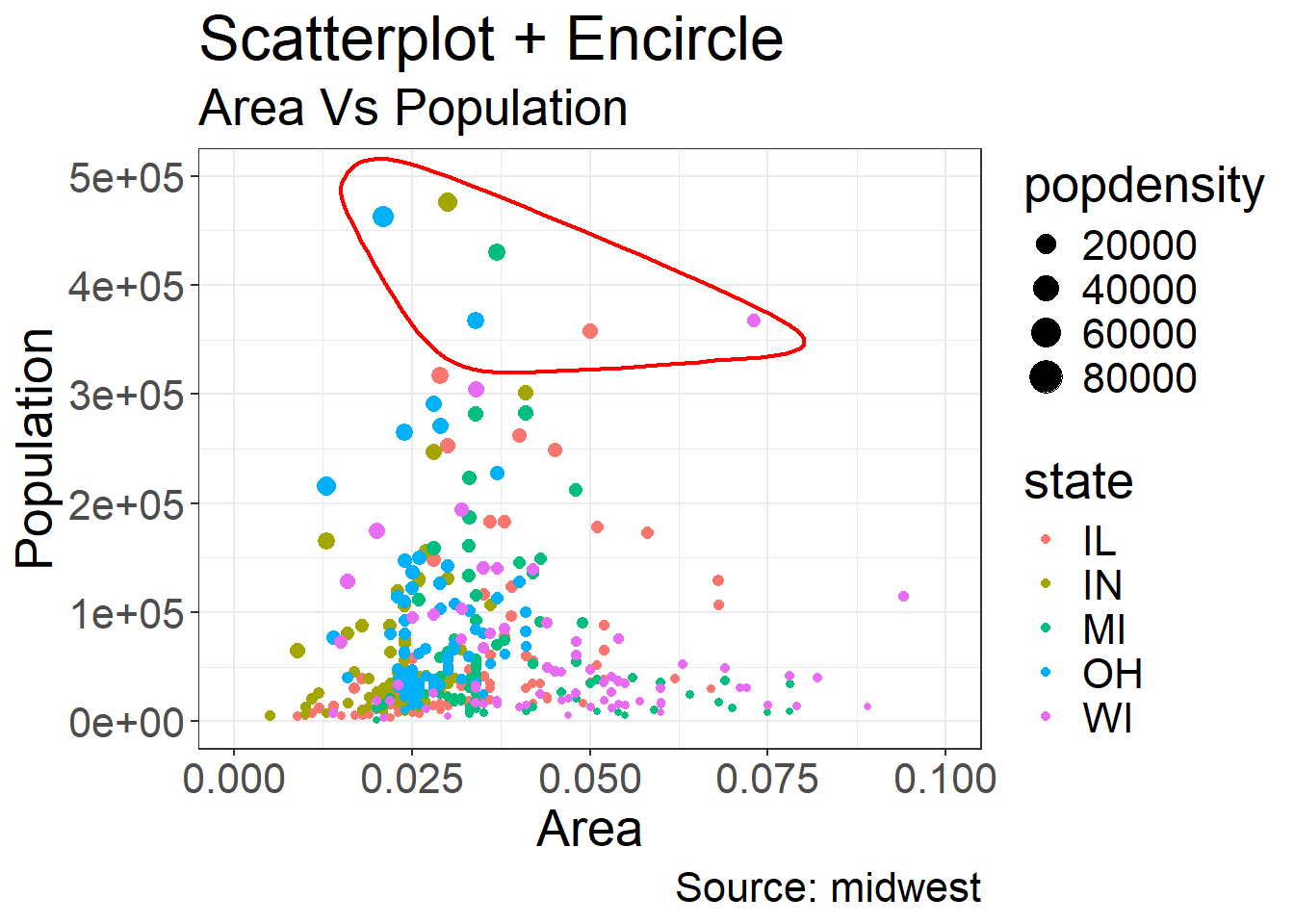
Coming back to the example we gave for “Other Aesthetics”, suppose that one is interested in emphasizing a certain area, then a range of dots can be circled

This is achieved by using geom_encircle in the ggalt package
Here we want to emphasize the observations where the population total is between 350k and 500k and where the area is between 0.01 and 0.1
Note that we need to find out these observations, which is done by creating the subset observations of midwest_select
We have also added the titles and caption

midwest_select <- midwest[midwest$poptotal > 350000 & 
                            midwest$poptotal <= 500000 & 
                            midwest$area > 0.01 & 
                            midwest$area < 0.1, ]

ggplot(midwest, aes(x=area, y=poptotal)) + 
  geom_point(aes(col=state, size=popdensity)) +   # draw points
  xlim(c(0, 0.1)) + 
  ylim(c(0, 500000)) +   # draw smoothing line
  geom_encircle(data=midwest_select, 
                color="red", 
                size=2, 
                expand=0.08) +   # encircle
  labs(subtitle="Area Vs Population", 
       y="Population", 
       x="Area", 
       title="Scatterplot + Encircle", 
       caption="Source: midwest") +
    theme(text = element_text(size=20)) #make axis/labels bigger
## Warning: Removed 15 rows containing missing values or values outside the scale range
## (`geom_point()`).

Reference

Advanced Example 3 - ggplot version

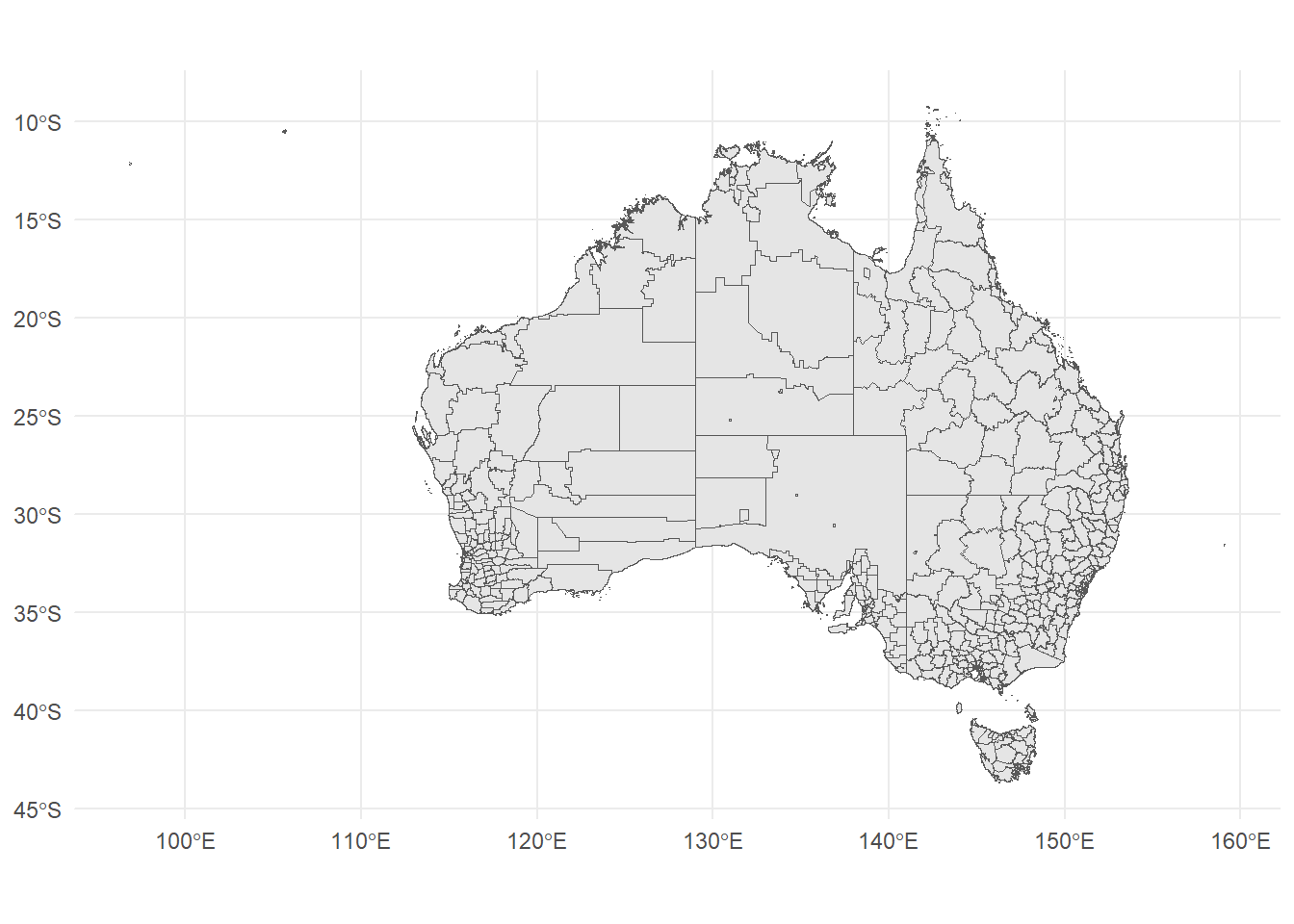
ggplot can also be used to create thematic maps to visualise data based on geography.

Advanced Example 3

The first step is to import map data. These kinds of datasets are called “shapefiles” because they are datasets that help programs like R draw shapes by spelling out complex polygons as a list of points. In this case the map is of Australia broken down into its Local Government Areas (LGA).

Note that the following five files are all required for this code to work:
- LGA11aAust.shp
- LGA11aAust.cpg
- LGA11aAust.dbf
- LGA11aAust.shx
- LGA11aAust.prj
This data can be found online on the ABS website where you can also find many other breakdowns of Australia, for example into postcode or statistical area levels.

Advanced Example 3

Once geometry data is found, we can use geom_sf (sf for shapefile) to create a map image:

Advanced Example 3

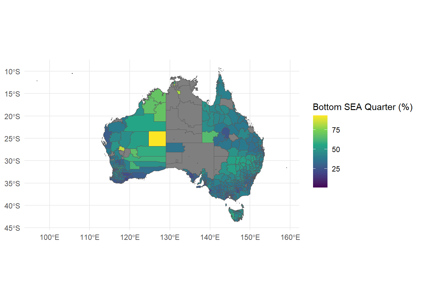
To make this graph informative, we then need some numerical data which is also grouped by LGA to plot on this map. heatmap_data.csv contains data on Index of Community Socio-Educational Advantage (ICSEA) by each LGA, so we need to merge this data with our shapefile data.

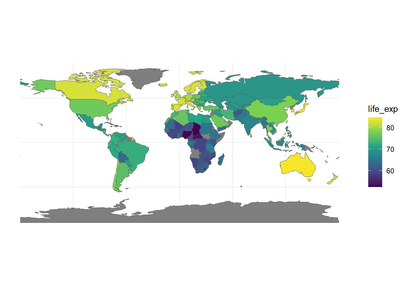
For those interested, when you are strictly making maps it can sometimes be better to use tmap which is more specifically designed for this task and comes with some nice default features.
However, it tends to have worse integration with the rest of the tidyverse.

Exercise

Use the world.gpkg data set to generate a map of the world using life expectancy as the scale. .gpkg files are another way of storing shapefile data other than the 5 file method you saw before but you can read it the same way using st_read(world.gpkg).

You can either download the dataset from Ed or by clicking here.

This data set is fully created by the publishers of tmap.

Solution

ggplot2 - Others

Use the last_plot() to returns the last plot you have created.
One can use the ggsave() function to save the last plot you have created.
One can use the function qplot() in a similar way as a traditional R plot function (but without the ‘plus sign’ synthax).

qplot(height,weight, data = raw_data)
## Warning: `qplot()` was deprecated in ggplot2 3.4.0.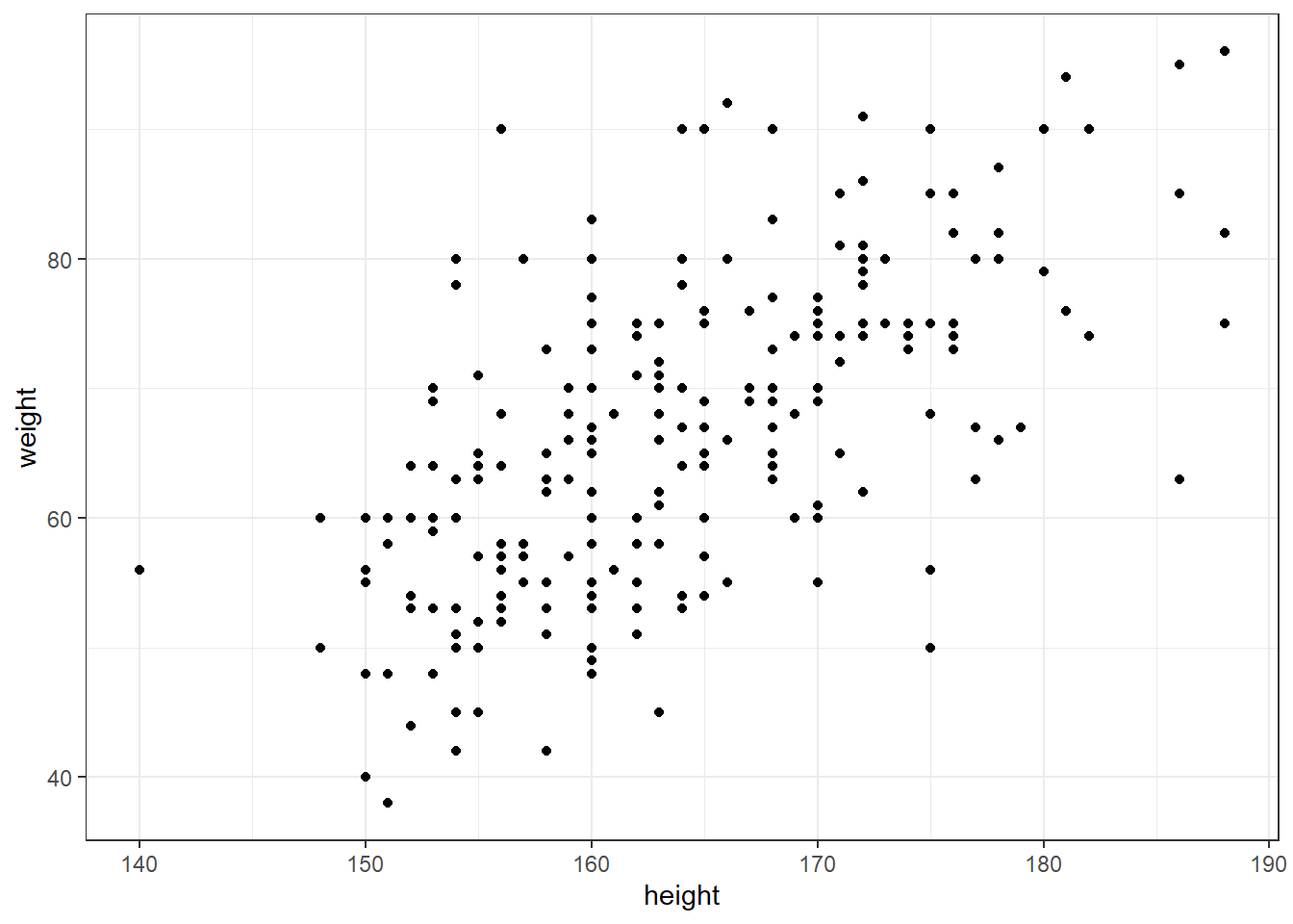

There are many more functions the ggplot2 package can offer. One can refer to the cheat sheet for more information.

Further Directions

Further Learning Directions

10 weeks unfortunately is simply not enough time to teach you all the amazing things that can be done with R.

With that in mind, the next slides will give you some ideas of various packages and frameworks you can look into if you are interested. These are all optional and just for those that are interested.

Obviously not all of these will interest all of you, but if there is one that you are intrigued by, then it is always a good idea to investigate further.

These are not in any particular order, some are very large and complex tools, and some are packages for some specific but useful purposes.

Smaller Packages

purrr and tidyr are two packages that are part of the tidyverse that can make your code much more efficient when used well. The first allows you to use functional programming within R (if you are unsure of what this is the website explains it a bit) and the second is for tidying and reshaping data.
tidyquant is a package that aims to take all of the previously popular financial analysis packages in R and implement them in a tidyverse way. This allows for greater integration of financial analysis with other tools like ggplot2.
plotly. While ggplot2 is excellent for static plots and has huge customisability, it tends to be difficult to create more “flashy” graphs like 3D plots or interactive plots. plotly aims to go the other way by having plots that are interactive, allowing for 3D plots, and by default including some “fancy” types of plots. You should go check out some examples on their site.

Smaller Packages continued

ggraph is an extension of ggplot2 which provides an easy way to create plots of relational data structures like networks, graphs and trees. This is definitely more of a specialty use case, but if you do need to draw graphs of graphs, this is an incredibly helpful package.
tidymodels is a package for modelling and machine learning, aiming to follow the tidyverse principles as well. This package may not be very useful yet as you would not have learned much about modelling (you have to wait for a course like ACTL3142 for that). However, once you are doing modelling, tidymodels is extremely well-designed and prevents the need for using a ridiculous number of packages all to do slightly different things.

Packages for Working with Data

data.table is a tool for manipulating large datasets. It performs a similar purpose to dplyr but with a couple of key trade-offs. data.table tends to have more confusing and unintuitive syntax and is not well integrated with the rest of the tidyverse. However, it is significantly faster than dplyr, particularly on large datasets, and is very memory efficient. If you are working with large datasets, it is worth looking into.
(Significantly more advanced) If you are really looking for a challenge and something new, learning how to work with proper databases is a very useful skill for anyone involved with data science. For those who want a (useful) challenge, here it is:
- While R can work with large datasets, at a certain point it becomes difficult and databases are significantly more efficient.
- The bright side is that the most popular language for databases is SQL, which is extremely similar to dplyr in how it functions (select, filter, group by, etc.).
- There are two main approaches to get started with databases (depending how comfortable you are with programming in general). If you are fairly comfortable and want to learn how to use databases “separately” to R feel free to look into SQLite, but for the majority that are not as comfortable and want to learn how to use databases within R, the R4DS textbook has a great introduction to databases through R, linked here.
- Once you have worked through the R4DS textbook there are plenty of other resources online (which become more accessible once you know the basics).

Typesetting

Most of you have probably heard of \(\LaTeX\) from MATH1151. For those which have not, it is a typesetting language that researchers use to write their papers and theses. It is a powerful tool that allows you to create beautifully formatted documents with extremely more control than a word processor like Microsoft Word or Google Docs. \(\LaTeX\) is not the focus of this slide but it is also very useful for the future, so a tutorial to get started is linked here.
Now that we have your interest in typesetting, we can introduce RMarkdown, which is a tool that allows you to write documents using parts of the \(\LaTeX\) engine, but more importantly allows you to embed R code that can be run into your documents. This allows you to create documents that can be easily updated with new data or new code, and the results will automatically update in the document. Demonstrating its abilities is best done through examples, so please check out the gallery and if you are interested in learning more this page has many places for you to get started (as always, it is R4DS to the rescue :)).
While RMarkdown is a great tool for writing documents, it is not the only one. Quarto is a multi-language, next generation version of R Markdown from the same people who made RStudio, R Markdown and Shiny. Quarto is much more flexible and powerful than R Markdown. In fact, the entire course website and slides for this course are all made with Quarto! Surely that must give you some motivation to learn it! Quarto effectively combines many popular tools for document/website/presentation creation and allows you to use them all in one. This means you can create websites using Shiny or ReactJS, presentations using Beamer or RevealJS, articles/books using Typst or \(\LaTeX\), dashboards and many more. As usual, examples show it best, and for getting started yet again it is R4DS that will serve you best. Once you understand the basics, the Quarto website has many guides to get you started with more complex use cases.

Shiny

A Shiny app is used to create web applications that incorporate interactive visualisations. It is hard to explain the full capabilities of Shiny, so you are better off looking at some examples.

There are plenty of examples on the Shiny Gallery, which is a great place to start.
In particular for some more “full demos” scroll down to the “User Showcase” section.
A couple of nice examples to look at are Example 1 and Example 2.

You can find a good introduction to Shiny app on the official website of R Studio:

Here is a course on Shiny, by one of the authors of your R book (Pierre Lafaye de Micheaux):

Link 3

Homework

Homework exercise I

Use the mtcars dataset in R and present the histogram and empirical distribution of the variable mpg.

Solution

# the number of bins needs to be relatively small here
# given the small size of sample
# log-transformation is not necessary here

ggplot(mtcars, aes(mpg))+geom_histogram(bins=5) # histogram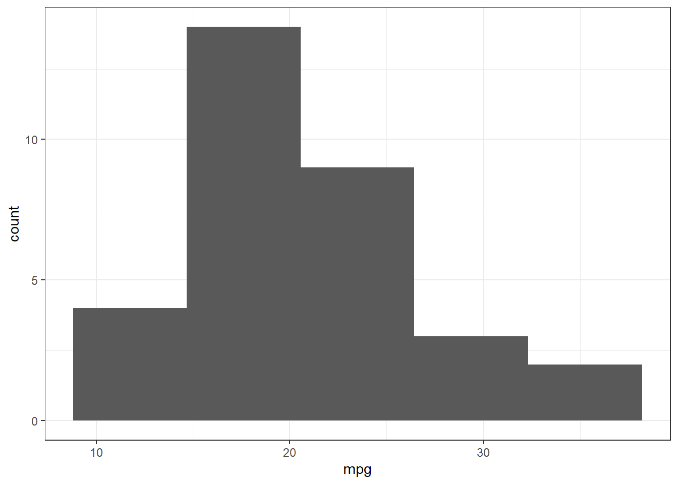


ggplot(mtcars, aes(mpg))+stat_ecdf() # empirical distribution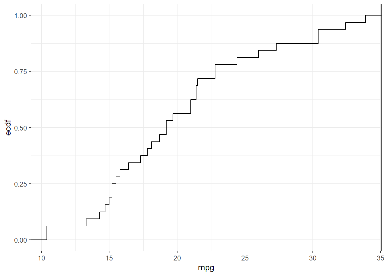

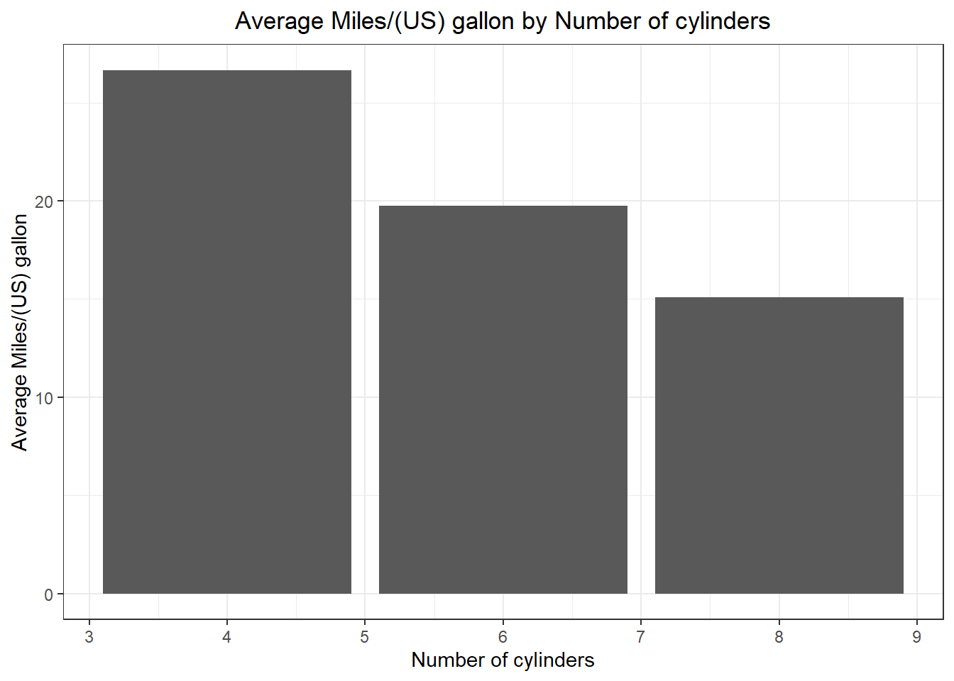
Homework exercise II

Use the mtcars dataset in R and present the average Miles/(US) gallon for each Number of cylinders.

Solution

# aggregate mpg given cyl
# the function we are interested in mean
mpg_cyl <- aggregate(mpg~cyl, mtcars, mean)

# create the bar plot
ggplot(mpg_cyl, aes(cyl, mpg))+ 
  geom_bar(stat = "identity") + 
  labs(x = "Number of cylinders", y = "Average Miles/(US) gallon") + 
  ggtitle("Average Miles/(US) gallon by Number of cylinders")+
  theme(plot.title = element_text(hjust = 0.5))