Week 3: Control flows and functions

Learning outcomes

By the end of this topic, you should be able to

create control flows in R
understand the concept and benefit of vectorization
call functions in R with specified arguments
create R functions (with and without default values)
learn how to use new functions using the help menu

Control Flow

Control Flow - Introduction

Code Academy: “Control flow refers to the order in which statements and instructions are executed in a program. It determines how the program progresses from one instruction to another based on certain conditions and logic.”

An ‘if’ statement is used to execute a command if some condition is satisfied.
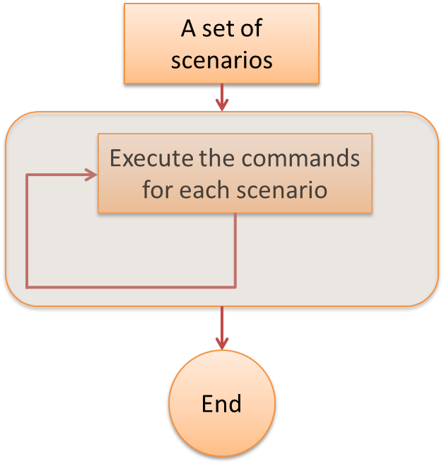
A loop can be used to repeat the same portion of code (or block of code) a number of times.
A ‘for’ loop is used to repeat a building block a pre-determined number of times.
A ‘while’ loop is used to repeat a building block until some condition fails.
In an algorithm, logical operations are used to decide whether a loop should continue or not.

Note: We will come back to the notion of ‘Algorithm’ in much more detail in Week 7.

Control Flow - `if` and `else` - Page 117

if and else if statements have the general syntax

if (condition) {
  something()
} else if (condition2) {
 somethingelse()
} else {
  otherwise()
}

The order of operations from R’s perspective is

Check condition, if TRUE execute something() and finish
If condition = FALSE, check condition2, if TRUE execute somethingelse() and finish
If both conditions are false, execute otherwise() and finish

Make sure your understand the above general structure “intuitively”; this kind of control is essential in programming. See also the example below.

x <- 3
y <- 4
if (x<y) {
  print("x smaller than y")
} else if (x==y){
  print("x equals y")
} else {
  print("x larger than y")
}

[1] "x smaller than y"

Note that it is possible to chain together as many else if’s as you want.
Furthermore, it is not strictly required to use else. I.e., you can get away with only if’s, but that is not efficient. Do you see why?

Control Flow - `for` - Page 119

A for loop has the general syntax

for (item in vector) {
  dosomething()
}

To execute this, R will run dosomething() for every item in vector (setting item to whichever one it is up to, at each iteration of dosomething()).

A simple example is the following

total = 0
for (x in c(3,7,11,13,17)) { # first few prime numbers
  total = total + x
  print(x)
}

[1] 3
[1] 7
[1] 11
[1] 13
[1] 17

total # after the loop has ended, show the total

[1] 51

Again, try to understand the general structure intuitively: for each item x in some vector, run this loop.

Exercise: For loop

Suppose you open a new bank account. At time $0$, you deposit $\$500$ into your account. Your account earns $i\%$ per annum of interest in year $i$ (i.e. $1\%$ in the first year, $2\%$ in the second year, etc.)

What would be your account balance at the end of the 10th year? Use a ‘for’ loop in your solution.

balance <- 500
for (i in 1:10) {
  balance <- balance*(1 + i/100)
}
balance

[1] 850.9107

Control Flow - `while` - Page 119

A while loop has the general syntax: while (condition){}
It repeats whatever commands are inside brackets {} as long as condition is TRUE.

x <- 2
y <- 1
while(x+y < 6) {
  x <- x+y
  print(x+y)
}

[1] 4
[1] 5
[1] 6

[1] 5

# (x=2,y=1) -> (x+y=3<6) -> (x=3,y=1) -> (x+y=4<6) -> 
#(x=4,y=1) -> (x+y=5<6) -> (x=5,y=1) -> (x+y=6) -> End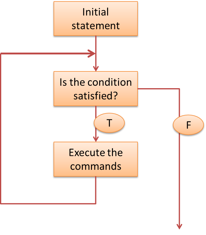

Exercise: While loop

With the help of function rpois(n=1, lambda = 2), generate a series of $\text{Poisson}(2)$ random variables $X_1, X_2, X_3, \ldots$ until one of them is equal to $5$. Store those random variables and display the full sequence.

X <- rpois(n=1, lambda = 2) # We generate our first random variable
X.vector <- X # To start with, our sequence only contains one result (X)
while (X != 5) {
  X <- rpois(n=1, lambda = 2) # We generate a new random variable
  X.vector <- c(X.vector,X) # We add it to the sequence
}
X.vector

[1] 4 4 5

Aside on `{}`

Hopefully this part of the slides has demonstrated the importance of the braces in writing code. Not only does it visually organise your code, but it also tells R which parts of your code belong to what.

One of the most common errors you will encounter in your coding journey is:

for (i in 1:10) {
  if (i > 4) {
    print("I am bigger than 4")}
  }
}

Error in parse(text = input): <text>:5:1: unexpected '}'
4:   }
5: }
   ^

See if you can work out what caused the error and how to fix it.

Notes

While in many other programming languages, loops are heavily used, in R the “standard advice” is that you should generally avoid them whenever possible. Simply put, this is due to the inbuilt vectorisation within R, and you can see an example of this on the next slide.
That said, with newer versions of R, there is some debate in the R community about how “bad” loops are, see here an interesting defence of loops.
Note that other control flow statements exists: break can be used to exit a loop, and next moves to the next iteration within a loop. See more info and examples on Pages 119-120 or here.

Vectorization - Pages 85-86

As we have already seen, R ‘naturally’ operates on vectors and matrices, without needing loops.
Some examples:

x <- c(1,2,3,4)
y <- c(5,6,7,8)
x + 5

[1] 6 7 8 9

sqrt(x)

[1] 1.000000 1.414214 1.732051 2.000000

x+y

[1]  6  8 10 12

M <- matrix(1:9, nrow=3)
exp(M)

          [,1]      [,2]     [,3]
[1,]  2.718282  54.59815 1096.633
[2,]  7.389056 148.41316 2980.958
[3,] 20.085537 403.42879 8103.084

sum(M)

[1] 45

We call this behaviour ‘vectorization’, and it is one of the main strengths of R.
Vectorization is usually much quicker than using loops!

Vectorization - Example - Pages 86

n <- 10^8
x <- runif(n) # Generate 100 million random elements 
z <- 0
system.time(for(i in 1:n){z <- z + x[i]}) # find their sum with a loop

   user  system elapsed 
   1.71    0.00    1.74

[1] 49998438

system.time(zz <- sum(x)) # find their sum with vectorization

   user  system elapsed 
   0.09    0.00    0.08

zz

[1] 49998438

Vectorization - helpful functions

Many functions in R apply to all items of a given vector, and also return a vector. We have seen examples of this already, e.g., sqrt(), log().
Knowing and using those functions should make your life easier.
While you can perform most tasks in a “custom” manner (using vectorization or not), the resulting syntax is often clunky/cumbersome.
Consider the following example: from a given vector, we want to double all even entries, and half all odd entries.

x <- c(1, 2, 4, 7, 8)

There are at least three ways to go about this

# 1. Using a for loop (inefficient)
# 2. Using simple vectorization and logical masks (okay but quite verbose), e.g.,
y <- x
y[y %% 2 == 0] <- 2 * y[y %% 2 == 0]
y[y %% 2 == 1] <- 0.5 * y[y %% 2 == 1]
y

[1]  0.5  4.0  8.0  3.5 16.0

# 3. Using the ifelse() function
(y <- ifelse(x %% 2 == 0, 2 * x, 0.5 * x))

[1]  0.5  4.0  8.0  3.5 16.0

The ifelse function is an internally vectorized function that checks if each item in a vector satisfies the condition in the first argument (x %% 2 == 0). If it does, it returns the second argument (2 * x), if it does not, it returns the third (0.5 * x).
There are other functions that similarly aim to minimise the use of loops via internal vectorization. Consider pmax

x <- c(2,5,7)
y <- c(3,4,8)
# I want to check, for each pair of elements, which is bigger, i.e. max(2,3), max(5,4) and max(7,8)
max(x, y) # this doesn't work, see if you can work out why, and what it actually does

[1] 8

pmax(x, y) # this returns the expected result, without using a loop

[1] 3 5 8

pmax(x, 6) # this usage is also quite common

[1] 6 6 7

Bottom line: before using a loop in R (which is not a crime, sometimes you have to), ask yourself:

is there an already existing function that can be used to do this task?
can I use an alternative “custom” syntax that exploits vectorization, hence avoids a loop?
can I create my own function to perform this task?

Functions

Calling functions - pages 43-44

A function in R is defined by its name and by the list of its parameters (or arguments). Most functions output a value.
Using a function (or calling or executing it) is done by typing its name followed, in brackets, by the list of arguments to be used. Arguments are separated by commas. Each argument can be followed by the sign = and the value to be given to the argument.

functionname(arg1 = value1, arg2 = value2, arg3 = value3)

Note that you do not necessarily need to indicate the names of the arguments, but only their values, as long as you follow their order.
For any R function, some arguments must be specified and others are optional (because a default value is already given in the code of the function).
Can you name some functions you already know and that we have seen?

Functions - calling functions - page 44

For the purposes of illustration we will use the log function, and if you check the help menu (more on this later), its usage is specified as log(x, base = exp(1)) where x is the value we are taking the log of, and base is of course the base of the log.

log(x, base = exp(1)) indicates that x is a required argument because it has no default, while base is optional, and will default to exp(1).

To start with we can run

log(x = 5, base = exp(1))

[1] 1.609438

Note that, as long as our ordering of arguments is the same as specified in the description of the function (via the help menu), we can omit the names:

log(5, exp(1))

[1] 1.609438

But, careful with this, you need the correct order. For example, this will give you a different (wrong) result:

log(exp(1), 5)

[1] 0.6213349

You may have noticed that in the usage specification, it says base = exp(1). This means the default argument for base is already exp(1). This means we can further simplify to

log(5)

[1] 1.609438

That covers most of the normal use cases. But we can extend this to some other ways of calling the function:

log(base = exp(1), 5) # Because we named the first one, it assumes the next is x

[1] 1.609438

log(b = exp(1), 5) # You can put part of the argument name as long as it is unambiguous

[1] 1.609438

Default arguments vs. no arguments

An important distinction between types of functions can be seen by calling

seq()

[1] 1

date()

[1] "Fri Jul 18 17:30:58 2025"

Both of these work without any arguments supplied, but they have a key distinction. seq has default values for all of its arguments, while date actually has no arguments.

We provide more details on seq later on.

Developing your own functions

Creating a function - Page 194

An important part of coding in R is creating your own functions. Indeed, whenever you are performing the same task many times (only with potentially different inputs each time), it is much better to create a custom function than to copy-paste your code (and then manually change the inputs for each iteration of the task).
Custom functions avoid copy-pasting errors. They make your code cleaner, easier to debug and easier to update/improve.
Creating a function is done following the general syntax: function(<list of arguments>){<body of the function>}, where
- <list of arguments> is a list of named arguments (also called formal arguments) ;
- <body of the function> represents, as the name suggests, the contents of the code to execute when the function is called.

Calling a function - Pages 194-195

To execute it, the user needs to call the function, followed by the effective arguments listed between brackets () and separated by commas. Here an effective argument is the value affected to a formal argument.

# This line creates a function called 'hello' with one argument called 'name'
hello <- function(name) {
  cat("Hello, my dear", name, "!") # cat is a function that joins strings together
}
# This line executes the function, with the the effective argument 'Josephine'
hello(name = "Josephine")

Hello, my dear Josephine !

Again, this can be called in different ways:

hello(na="Jinxia")

Hello, my dear Jinxia !

hello(n="Samantha")

Hello, my dear Samantha !

hello("Bernard")

Hello, my dear Bernard !

Developing functions - Body of a function - Page 195

The body of a function can be a simple R instruction, or a sequence of R instructions. In the latter case, as mentioned before, the instructions must be enclosed between the characters { and } to delimit the beginning and end of the body of the function.
Several R instructions can be written on the same line as long as they are separated by a semicolon ‘;’ (while you can do this, it is generally not advisable as it tends to be less readable).

Exercise - Page 195

Create a function called favourite() such that there is a single argument called course, and the function returns "My favourite university subject is {course}!". The default argument of course should be set to "ACTL1101", obviously :-).

Expected behaviour:

> favourite()
My favourite university subject is ACTL1101!

> favourite("actl2131")
My favourite university subject is ACTL2131!

Hint: use toupper()

Solution:

favourite <- function(course="ACTL1101") {
  return(paste("My favourite university subject is ", toupper(course), "!", sep = "")) 
  # paste also joins strings together
  # the argument sep indicates the separator between each item
}
favourite("actl2131")

[1] "My favourite university subject is ACTL2131!"

favourite()

[1] "My favourite university subject is ACTL1101!"

Developing functions - Multiple arguments example

Of course, a function can have more than one argument. Here, function CDF.pois() has two arguments, x and lambda. It calculates the CDF $F_X(x)$ at x of a Poisson random variable with parameter equal to lambda. Note the use of a for loop.

CDF.pois <- function(x, lambda){
  # Initialise the cdf to 0
  cdf = 0
  # For k from 0 to x, add together the probablity masses p(k)
  for (k in 0:x){
    cdf = cdf + exp(-lambda)*lambda^k/factorial(k)
  }
  # Return the result
  return(cdf)
}
CDF.pois(x = 3, lambda = 4)

[1] 0.4334701

Note: we have every right to use a function within a function. For instance, here we used the (already defined) function factorial() inside our new function CDF.pois().

Developing functions - Exercise - pages 45-46

Code a function which takes two arguments $n$ and $p$ and calculates the binomial coefficient \[{n \choose p}=\frac{n!}{p!(n-p)!}\]

Test your function by evaluating the result of \[{5 \choose 3}\] which should yield $10$.

Solution:

binomial <- function(n,p) {factorial(n)/(factorial(p)*factorial(n-p))}
binomial(5,3)

[1] 10

Developing functions - Default argument values - Page 195

When declaring a function, all arguments are identified by a unique name.
Each argument can be associated with a default value. To specify a default value, use the character = followed by the default value.
When the function is called with no effective argument for that argument, the default value will be used.

# Declare function 'binomial' with default values
binomial <- function(n=5,p=3){factorial(n)/(factorial(p)*factorial(n-p))}

binomial() # Use both default values

[1] 10

binomial(n=6) # Specify first argument, but use default value for the second

[1] 20

Developing functions - Object returned by a function - Pages 198-199

A way to explicitly tell an R function what object to return is to use the function return(). This instruction halts the execution of the code in the body of the function and returns the object between brackets.

binomial <- function(n=5,p=3){
  return(factorial(n)/(factorial(p)*factorial(n-p)))
  # Everything below will NOT be executed, because we returned the first part
  my.unif <- runif(1)
  while (my.unif <= 1){ # Note that this part would be an infinite loop! Beware of those!
    my.unif <- runif(1)
  }
}

If there is no ‘return()’ in the body of the function, then the function will return the result of the last evaluated expression.

Developing functions - Variable scope in the body of a function - Page 200-201

Variables defined inside the body of a function have a local scope during function execution. This means that a variable inside the body of a function is different from another variable with the same name, but defined in the workspace of your R session.
Generally speaking, local scope means that a variable only exists inside the body of the function. After the execution of the function, the variable is thus automatically deleted from the memory of the computer.
While this behaviour may seem strange, it is usually a good thing because it keeps the clutter of all objects defined in a function away from our overall environment.

Exercise

Create a function in R that calculates the present value of an annuity (paying $1$ per year). The inputs are

the number of years, which is by default $1$
whether the payments are paid in arrears or not, which is by default TRUE
the annual interest rate, which is by default $6\%$

Note: recall that the present value of an annuity that pays $1$ at the end of each year for $n$ years is \[\frac{1-(1+i)^{-n}}{i}.\] If payments occur at the beginning of the year (rather than in arrears), then the present value is \[(1+i)\frac{1-(1+i)^{-n}}{i}.\]

Solution

annuity_cal <- function(n=1, arrears=TRUE, i=0.06){
  discount <- 1/(1+i)
  temp <- (1-discount^n)/i
    if (arrears == T){
      return(temp)
    }
    else{ 
      return(temp*(1+i))
    }
}

annuity_cal()

[1] 0.9433962

annuity_cal(a=FALSE)

[1] 1

annuity_cal(n=5, a=FALSE, i=0.07)

[1] 4.387211

Exercise

Create a function in R that plots the density or distribution function of a normal random variable. The arguments are

mean $\mu$, which is by default 0
variance $\sigma^2$, which is by default 1
whether a density function is plotted, which is by default TRUE; if FALSE, then the cumulative distribution function is plotted

The output is either the density or the distribution function over the range $(\mu-4\sigma,\mu+4\sigma)$.

Hint: You will need functions dnorm() and pnorm() as well as function plot().

Note: There is more to come about graphical tools in Weeks 5.

Solution

Note: you can scroll down for more examples.

plot_norm <- function(mean=0, variance=1, density=TRUE) {
  temp <- seq(from=mean-4*sqrt(variance), to=mean+4*sqrt(variance), by=sqrt(variance)/50)
  
  if (density) { # Note writing 'if (density)' is equivalent to writing 'if (density = T)' 
    plot(temp, dnorm(temp, mean, sqrt(variance)))
  } else {
    plot(temp, pnorm(temp, mean, sqrt(variance)))
  }
}
plot_norm()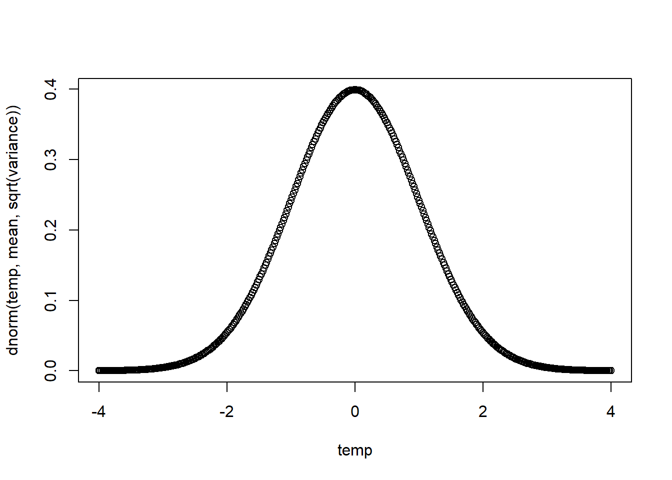

plot_norm(1,4,TRUE)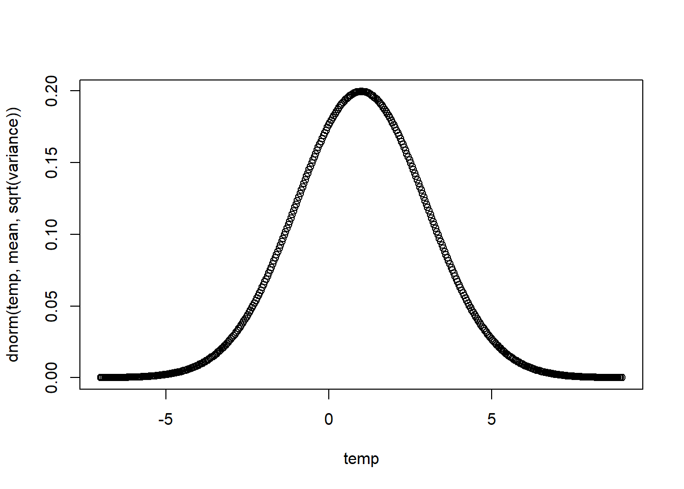

plot_norm(1,4,FALSE)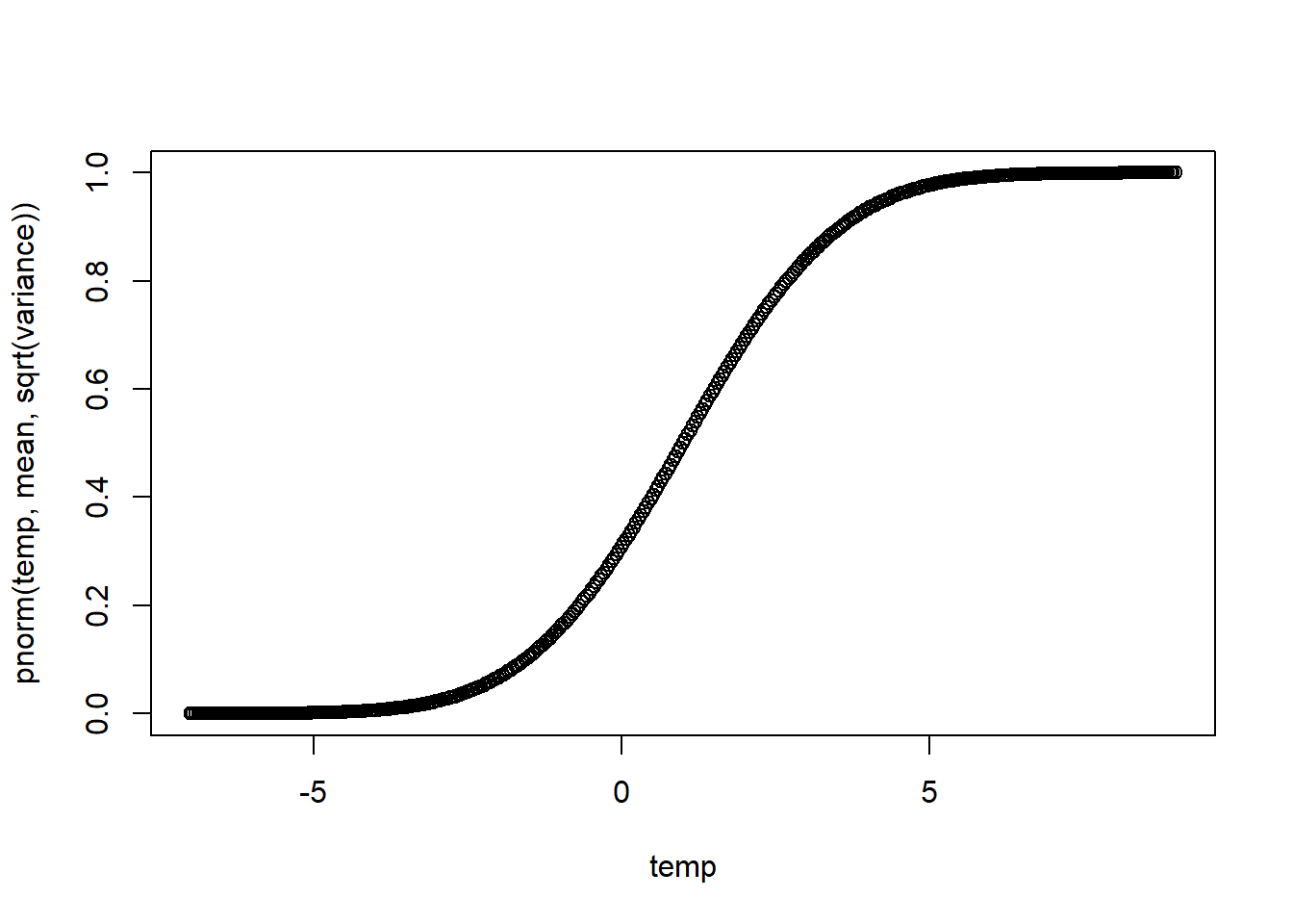

Help Menu

The `help` menu - `seq`

As an example, let’s look at the function seq(), which generates a sequence of numbers between two numbers.
You can read the documentation for seq either by typing help(seq) in RStudio, or clicking here

The documentation can be broken down into a few sections

Description: this is just a brief overview of what the function is intended to do
- for seq it says it generates regular sequences
Usage: this shows you how to use the functions and importantly what arguments it takes and what their default values are
- for seq the key ones are from, to, by, and length.out, while the first two might be obvious, the latter two may not be.
Arguments: this tells you exactly what the arguments should be and what effect they have
- We can see from and to describe the start and end points of the sequence.
- We then see that by is the common increment and length.out is how many points to divide the sequence into. If these seem overlapping, it is because they are (you should only specify one of these two). You may also note that the default argument of by is calculated from length.out. Do you see the logic of this formula?
Values: this tells you what the function will output
- For seq it says it outputs a vector
- The Values section for seq is quite simple, but in more advanced functions there will be several outputs that all describe different things
Details: this describes any extra details of the function’s behaviour and normally describes how it works internally
Examples: this is possibly the most important section, as it shows you some common usages of the function. Once you become familiar with programming, learning by example will likely become your preferred method

Homework

Homework Exercise 1

Using a ‘for’ loop, find how many positive integers less than a million are divisible by both $8$ and $42$.

Hint: Use the modular division which has syntax x %% y (and gives you the remainder of the division x / y), see examples below.

4 %% 3

[1] 1

3 %% 4

[1] 3

4 %% 2

[1] 0

Homework Exercise 2

Using a ‘while’ loop, find the lowest common multiple of $120$ and $46$.

Homework Exercise 3

Create a function with one argument called m (taking default value $10$) and one argument called lambda (with no default value). This function should generate a sequence of size m from Poisson random variables (each with parameter lambda). The function should then return all the even values hence generated.

Hint: modular division could again be helpful.

Homework Exercise 4

If we start at $1$, how many consecutive natural numbers $(1,2,3,4, \ldots)$ do we need to multiply together to get a number greater than $500,\!000$?

Homework Exercise 5

The Collatz sequence goes as follows: start at any positive integer, then

if the number is $1$, stop
if the number is even, divide it by $2$
if the number is odd, multiply it by $3$ and add $1$

It is conjectured but not proven that the sequence always reaches 1, eventually. For example, the Collatz sequence starting at $5$ is: \[ 5 \to 16 \to 8 \to 4 \to 2 \to 1\]

Create a function collatzNext() that takes in any positive integer and returns the next number in the Collatz sequence. For example, collatzNext(5) should return 16.

Create another function, collatzSequence() that takes in any positive integer and returns the full Collatz sequence starting from that integer and ending at $1$. For example, collatzSequence(5) should return 5 16 8 4 2 1. Hint: You may want to use collatzNext() in this function.

For both functions, set the default argument as $1$.

Learning outcomes

Control Flow

Control Flow - Introduction

Control Flow - if and else - Page 117

Control Flow - for - Page 119

Exercise: For loop

Control Flow - while - Page 119

Exercise: While loop

Aside on {}

Notes

Vectorization - Pages 85-86

Vectorization - Example - Pages 86

Vectorization - helpful functions

Functions

Calling functions - pages 43-44

Functions - calling functions - page 44

Default arguments vs. no arguments

Developing your own functions

Creating a function - Page 194

Calling a function - Pages 194-195

Developing functions - Body of a function - Page 195

Exercise - Page 195

Developing functions - Multiple arguments example

Developing functions - Exercise - pages 45-46

Developing functions - Default argument values - Page 195

Developing functions - Object returned by a function - Pages 198-199

Developing functions - Variable scope in the body of a function - Page 200-201

Exercise

Solution

Exercise

Solution

Help Menu

The help menu

The help menu - seq

Homework

Homework Exercise 1

Homework Exercise 2

Homework Exercise 3

Homework Exercise 4

Homework Exercise 5

Control Flow - `if` and `else` - Page 117

Control Flow - `for` - Page 119

Control Flow - `while` - Page 119

Aside on `{}`

The `help` menu

The `help` menu - `seq`