rownames(college) <- college[, 1]
View(college)Lab 1: Introduction To Statistical Learning
Questions
Conceptual Questions
\star (ISLR2, Q2.1) For each of parts (a) through (d), indicate whether we would generally expect the performance of a flexible statistical learning method to be better or worse than an inflexible method. Justify your answer.
The sample size n is extremely large, and the number of predictors p is small.
The number of predictors p is extremely large, and the number of observations n is small.
The relationship between the predictors and response is highly non-linear.
The variance of the error terms, i.e., \sigma^2 = \mathbb{V}(\epsilon), is extremely high.
(ISLR2, Q2.2) Explain whether each scenario is a classification or regression problem, and indicate whether we are most interested in inference or prediction. Finally, provide n and p.
We collect a set of data on the top 500 firms in the US. For each firm we record profit, number of employees, industry and the CEO salary. We are interested in understanding which factors affect CEO salary.
We are considering launching a new product and wish to know whether it will be a success or a failure. We collect data on 20 similar products that were previously launched. For each product we have recorded whether it was a
successorfailure, price charged for the product, marketing budget, competition price, and ten other variables.We are interested in predicting the % change in the USD/Euro exchange rate in relation to the weekly changes in the world stock markets. Hence we collect weekly data for all of 2012. For each week we record the % change in the USD/Euro, the % change in the US market, the % change in the British market, and the % change in the German market.
\star (ISLR2, Q2.3) We now revisit the bias-variance decomposition.
Provide a sketch of typical (squared) bias, variance, training error, test error, and Bayes (or irreducible) error curves, on a single plot, as we go from less flexible statistical learning methods towards more flexible approaches. The x-axis should represent the amount of flexibility in the method, and the y-axis should represent the values for each curve. There should be five curves. Make sure to label each one.
Explain why each of the five curves has the shape displayed in part (a).
\star (ISLR2, Q2.5) What are the advantages and disadvantages of a very flexible (versus a less flexible) approach for regression or classification? Under what circumstances might a more flexible approach be preferred to a less flexible approach? When might a less flexible approach be preferred?
\star (ISLR2, Q2.7) The table below provides a training data set containing six observations, three predictors, and one qualitative response variable.
Obs. X_1 X_2 X_3 Y 1 0 3 0 Red 2 2 0 0 Red 3 0 1 3 Red 4 0 1 2 Green 5 -1 0 1 Green 6 1 1 1 Red Suppose we wish to use this data set to make a prediction for Y when X_1 = X_2 = X_3 = 0 using K-nearest neighbors.
Compute the Euclidean distance between each observation and the test point, X_1 = X_2 = X_3 = 0.
What is our prediction with K = 1? Why?
What is our prediction with K = 3? Why?
If the Bayes decision boundary in this problem is highly non-linear, then would we expect the
bestvalue for K to be large or small? Why?
Applied Questions
\star (ISLR2, Q2.8) This exercise relates to the
Collegedata set, which can be found in the fileCollege.csvon Website homepage. It contains a number of variables for 777 different universities and colleges in the US. The variables arePrivate: Public/private indicatorApps: Number of applications receivedAccept: Number of applicants acceptedEnroll: Number of new students enrolledTop10perc: New students from top 10% of high school classTop25perc: New students from top 25% of high school classF.Undergrad: Number of full-time undergraduatesP.Undergrad: Number of part-time undergraduatesOutstate: Out-of-state tuitionRoom.Board: Room and board costsBooks: Estimated book costsPersonal: Estimated personal spendingPhD: Percent of faculty with Ph.D.’sTerminal: Percent of faculty with terminal degreeS.F.Ratio: Student/faculty ratioperc.alumni: Percent of alumni who donateExpend: Instructional expenditure per studentGrad.Rate: Graduation rate
Before reading the data into
R, it can be viewed in Excel or a text editor.Use the
read.csv()function to read the data intoR. Call the loaded datacollege. Make sure that you have the directory set to the correct location for the data.Look at the data using the
View()function. You should notice that the first column is just the name of each university. We don’t really wantRto treat this as data. However, it may be handy to have these names for later. Try the following commands:You should see that there is now a
row.namescolumn with the name of each university recorded. This means thatRhas given each row a name corresponding to the appropriate university.Rwill not try to perform calculations on the row names. However, we still need to eliminate the first column in the data where the names are stored. Trycollege <- college[, -1] View(college)Now you should see that the first data column is
Private. Note that another column labeledrow.namesnow appears before thePrivatecolumn. However, this is not a data column but rather the name thatRis giving to each row.Use the
summary()function to produce a numerical summary of the variables in the data set.Use the
pairs()function to produce a scatterplot matrix of the first ten columns or variables of the data. Recall that you can reference the first ten columns of a matrixAusingA[,1:10].Use the
plot()function to produce side-by-side boxplots ofOutstateversusPrivate.
Create a new qualitative variable, called
Elite, bybinningtheTop10percvariable. We are going to divide universities into two groups based on whether or not the proportion of students coming from the top 10% of their high school classes exceeds 50%.Elite <- rep("No", nrow(college)) Elite[college$Top10perc > 50] <- "Yes" Elite <- as.factor(Elite) college <- data.frame(college, Elite)Use the
summary()function to see how many elite universities there are. Now use theplot()function to produce side-by-side boxplots ofOutstateversusElite.Use the
hist()function to produce some histograms with differing numbers of bins for a few of the quantitative variables. You may find the commandpar(mfrow = c(2, 2))useful: it will divide the print window into four regions so that four plots can be made simultaneously. Modifying the arguments to this function will divide the screen in other ways.Continue exploring the data, and provide a brief summary of what you discover.
\star (ISLR2, Q2.9) This exercise involves the
Autodata set studied in the lab. Make sure that the missing values have been removed from the data.Which of the predictors are quantitative, and which are qualitative?
What is the range of each quantitative predictor? You can answer this using the
range()function.What is the mean and standard deviation of each quantitative predictor?
Now remove the 10th through 85th observations. What is the range, mean, and standard deviation of each predictor in the subset of the data that remains?
Using the full data set, investigate the predictors graphically, using scatterplots or other tools of your choice. Create some plots highlighting the relationships among the predictors. Comment on your findings.
Suppose that we wish to predict gas mileage (
mpg) on the basis of the other variables. Do your plots suggest that any of the other variables might be useful in predictingmpg? Justify your answer.
(ISLR2, Q2.10) This exercise involves the
Bostonhousing data set.To begin, load in the
Bostondata set. TheBostondata set is part of theISLR2library.library(ISLR2)Now the data set is contained in the object
Boston.BostonRead about the data set:
?BostonHow many rows are in this data set? How many columns? What do the rows and columns represent?
Make some pairwise scatterplots of the predictors (columns) in this data set. Describe your findings.
Are any of the predictors associated with per capita crime rate? If so, explain the relationship.
Do any of the census tracts of Boston appear to have particularly high crime rates? Tax rates? Pupil-teacher ratios? Comment on the range of each predictor.
How many of the census tracts in this data set bound the Charles river?
What is the median pupil-teacher ratio among the towns in this data set?
Which census tract of Boston has lowest median value of owneroccupied homes? What are the values of the other predictors for that census tract, and how do those values compare to the overall ranges for those predictors? Comment on your findings.
In this data set, how many of the census tracts average more than seven rooms per dwelling? More than eight rooms per dwelling? Comment on the census tracts that average more than eight rooms per dwelling.
Solutions
Conceptual Questions
Better: flexible models are better able to capture all the trends in the large amount of data we have.
Worse: flexible models will tend to overfit the small amount of data we have using the large number of predictors.
Better: inflexible models tend to have a hard time fitting non-linear relationships.
Worse: flexible models will tend to fit the noise, which is not desired.
Regression: the response (CEO salary) is continuous. Inference: We are interested in the factors influencing CEO salary – we don’t want to estimate it using a company’s information! n = 500 (500 companies in the data set) p = 3 (predictors: profit, number of employees, industry; response: CEO salary)
Classification: the response (success or failure) is discrete. Prediction: based on various input factors, we want to estimate how well the product will do n = 20 (20 similar products in the data set) p = 13 (predictors: marketing budget, price charged, competition price, +10 others; response: whether it was a success or failure)
Regression: the response (% change in US dollar) is continuous. Prediction: it’s written in the question! We are interested in predicting changes in the US dollar. n \approx 50 (number of trading weeks in a year) p = 3 (predictors: % change in US market, % change in UK market, % change in DE market; response % change in US dollar)
See the figure

image Bias: increasing flexibility reduces model bias
Training error: increasing flexibility makes the model fit the training data better
Variance: increasing flexibility makes the model incorporate more noise (in other words, it makes the fit bumpier)
Test error: concave up, since increasing flexibility makes the model fit more of the trend in the data until it starts fitting the noise in the data
Bayes’ (irreducible) error: horizontal line, since it’s a constant for all models. When the training error dips below the Bayes’ error, the model is overfitting, so the test error starts to increase
Advantages: can fit a larger variety of (non-linear) models, decreasing bias.
Disadvantages: can lead to overfitting (hence worse results), requires estimating more parameters, and increasing model variance as it incorporates more noise.
More flexible models would be preferred if the model is non-linear in nature, or interpretability is not a major issue. Less flexible models are preferred when inference is the goal of the model fitting exerciseSee the table below
Obs. X_1 X_2 X_3 Distance Y 1 0 3 0 3 Red 2 2 0 0 2 Red 3 0 1 3 \sqrt{10} \approx 3.2 Red 4 0 1 2 \sqrt{5} \approx 2.2 Green 5 -1 0 1 \sqrt{2} \approx 1.4 Green 6 1 1 1 \sqrt{3} \approx 1.7 Red Green. K=1 so we only take the closest observation (5).
K=3 so we consider the closest 3: 5, 6 and 2. The majority are Red, so this classifies as Red.
A smaller K would lead to a more flexible decision boundary, which would account for the non-linearity better.
Applied Questions
Refer to Section 2.3 of ISLR2 for a primer of applied questions.
Note that the dataset is available from the course Website homepage.
college <- read.csv("College.csv")The row names need to be changed to college names as follow
rownames(college) <- college[, 1] college <- college[, -1] college$Private <- as.factor(college$Private)head(college) # You should instead try `View(college)`summary(college)Private Apps Accept Enroll Top10perc No :212 Min. : 81 Min. : 72 Min. : 35 Min. : 1.00 Yes:565 1st Qu.: 776 1st Qu.: 604 1st Qu.: 242 1st Qu.:15.00 Median : 1558 Median : 1110 Median : 434 Median :23.00 Mean : 3002 Mean : 2019 Mean : 780 Mean :27.56 3rd Qu.: 3624 3rd Qu.: 2424 3rd Qu.: 902 3rd Qu.:35.00 Max. :48094 Max. :26330 Max. :6392 Max. :96.00 Top25perc F.Undergrad P.Undergrad Outstate Min. : 9.0 Min. : 139 Min. : 1.0 Min. : 2340 1st Qu.: 41.0 1st Qu.: 992 1st Qu.: 95.0 1st Qu.: 7320 Median : 54.0 Median : 1707 Median : 353.0 Median : 9990 Mean : 55.8 Mean : 3700 Mean : 855.3 Mean :10441 3rd Qu.: 69.0 3rd Qu.: 4005 3rd Qu.: 967.0 3rd Qu.:12925 Max. :100.0 Max. :31643 Max. :21836.0 Max. :21700 Room.Board Books Personal PhD Min. :1780 Min. : 96.0 Min. : 250 Min. : 8.00 1st Qu.:3597 1st Qu.: 470.0 1st Qu.: 850 1st Qu.: 62.00 Median :4200 Median : 500.0 Median :1200 Median : 75.00 Mean :4358 Mean : 549.4 Mean :1341 Mean : 72.66 3rd Qu.:5050 3rd Qu.: 600.0 3rd Qu.:1700 3rd Qu.: 85.00 Max. :8124 Max. :2340.0 Max. :6800 Max. :103.00 Terminal S.F.Ratio perc.alumni Expend Min. : 24.0 Min. : 2.50 Min. : 0.00 Min. : 3186 1st Qu.: 71.0 1st Qu.:11.50 1st Qu.:13.00 1st Qu.: 6751 Median : 82.0 Median :13.60 Median :21.00 Median : 8377 Mean : 79.7 Mean :14.09 Mean :22.74 Mean : 9660 3rd Qu.: 92.0 3rd Qu.:16.50 3rd Qu.:31.00 3rd Qu.:10830 Max. :100.0 Max. :39.80 Max. :64.00 Max. :56233 Grad.Rate Min. : 10.00 1st Qu.: 53.00 Median : 65.00 Mean : 65.46 3rd Qu.: 78.00 Max. :118.00Privateis not numerical, so cannot be used in pairs so we plot from column 2 onwardpairs(college[, 1:10])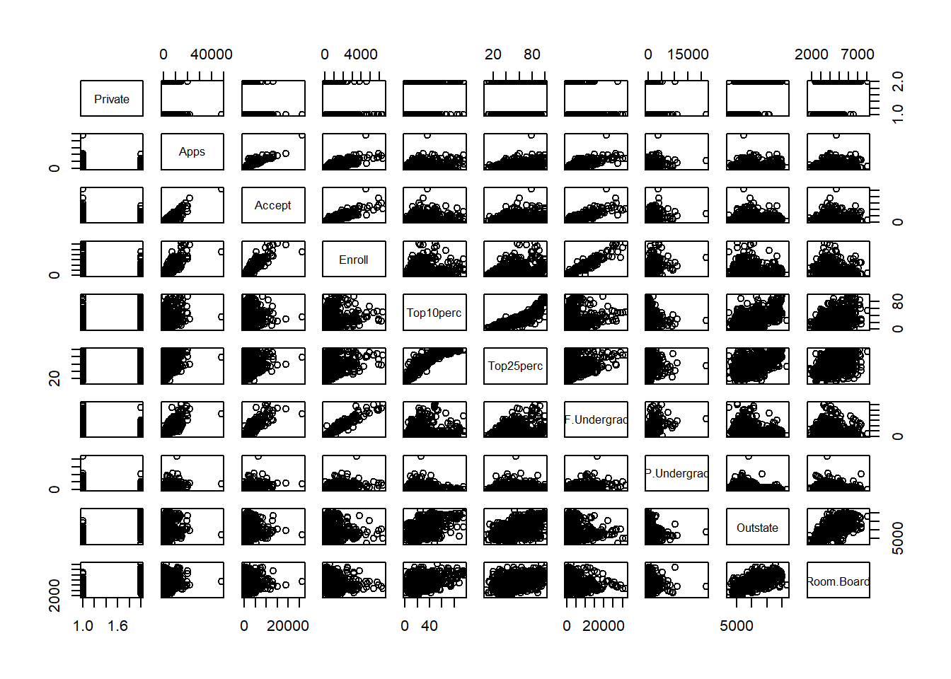
plot(college$Private, college$Outstate)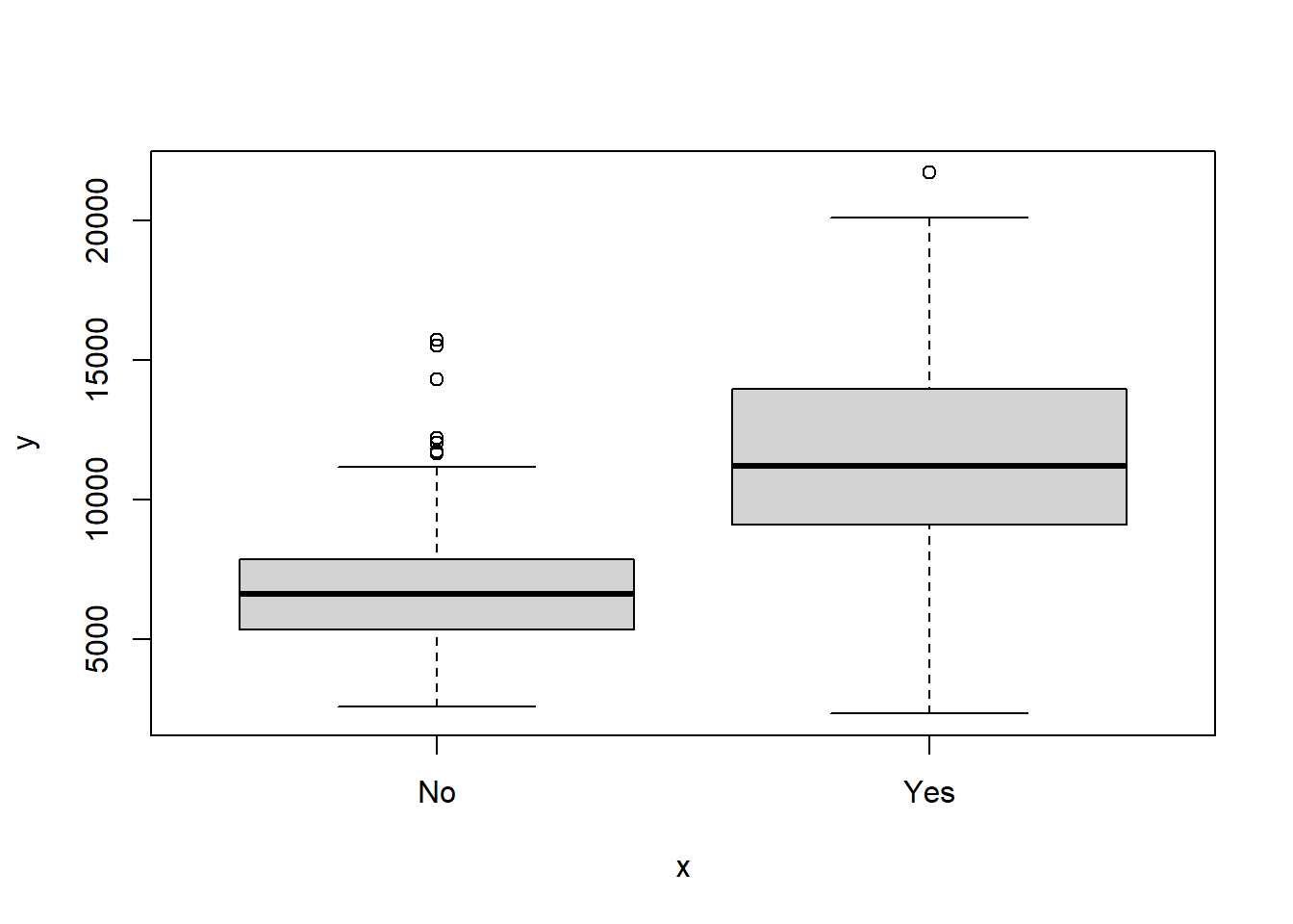
Elite <- with(college, ifelse(Top10perc > 50, "Yes", "No"))
Elite <- as.factor(Elite)
college <- data.frame(college, Elite)
summary(Elite) # there are 78 elite universities
No Yes 699 78plot(college$Elite, college$Outstate)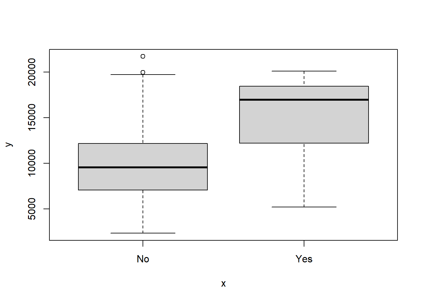
For instance the following code gives histograms for variables
Apps,Accept,Top10percandTop25perc.par(mfrow = c(2, 2)) hist(college$Apps, breaks = 20) hist(college$Accept, breaks = 20) hist(college$Top10perc, breaks = 20) hist(college$Top25perc, breaks = 20)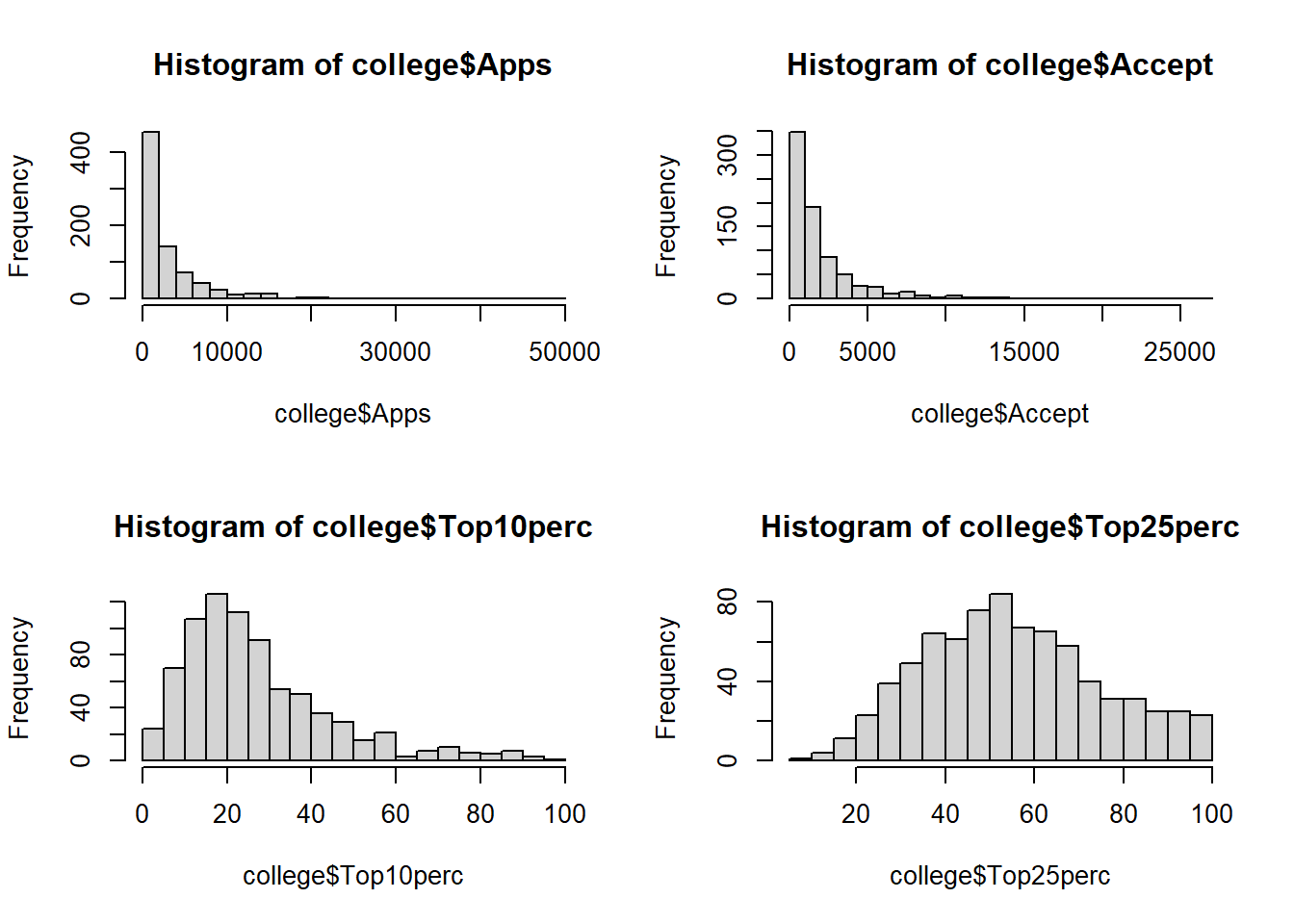
Note that the dataset is available from the course Website homepage.
auto <- read.csv("Auto.csv", na.strings = "?")
auto <- na.omit(auto) # remove missing values
Qualitative:
name,origin. Quantitative:mpg,cylinders,displacement,horsepower,weight,acceleration,year.We can use function
applycombined with functionrange:quant.var <- c( "mpg", "cylinders", "displacement", "horsepower", "weight", "acceleration", "year" ) ranges.df <- apply(auto[, quant.var], 2, range) rownames(ranges.df) <- c("min", "max") ranges.dfmpg cylinders displacement horsepower weight acceleration year min 9.0 3 68 46 1613 8.0 70 max 46.6 8 455 230 5140 24.8 82Use a similar application of function
apply:means.df <- apply(auto[, quant.var], 2, mean) std.df <- apply(auto[, quant.var], 2, sd) distns.df <- rbind(means.df, std.df) rownames(distns.df) <- c("mean", "sd.") t(distns.df)mean sd. mpg 23.445918 7.805007 cylinders 5.471939 1.705783 displacement 194.411990 104.644004 horsepower 104.469388 38.491160 weight 2977.584184 849.402560 acceleration 15.541327 2.758864 year 75.979592 3.683737Semantic note: the following will remove the 10th to the 85th row, which may not be what we want, since we have already removed some rows to begin with:
subauto <- auto[-(10:85), ]You will find that observation #86 has errantly been removed. That is because the
na.omitfrom earlier removed an observation in this range. It is possible to refer to the rows by observation number, which is a character string. In other words,auto["5",]will give me observation #5, even if 1-4 are missing. This does complicate the procedure, though.rid <- rownames(auto) rid <- rid[as.numeric(rid) < 10 | as.numeric(rid) > 85] subauto <- auto[rid, ]Use
applyfunction:subranges.df <- apply(subauto[, quant.var], 2, range) submeans.df <- apply(subauto[, quant.var], 2, mean) substd.df <- apply(subauto[, quant.var], 2, sd) subdistns.df <- rbind(subranges.df, submeans.df, substd.df) rownames(subdistns.df) <- c("min", "max", "mean", "sd.") t(subdistns.df)min max mean sd. mpg 11.0 46.6 24.368454 7.880898 cylinders 3.0 8.0 5.381703 1.658135 displacement 68.0 455.0 187.753943 99.939488 horsepower 46.0 230.0 100.955836 35.895567 weight 1649.0 4997.0 2939.643533 812.649629 acceleration 8.5 24.8 15.718297 2.693813 year 70.0 82.0 77.132492 3.110026For instance a pairwise plot can be produced using:
pairs(auto[, -9])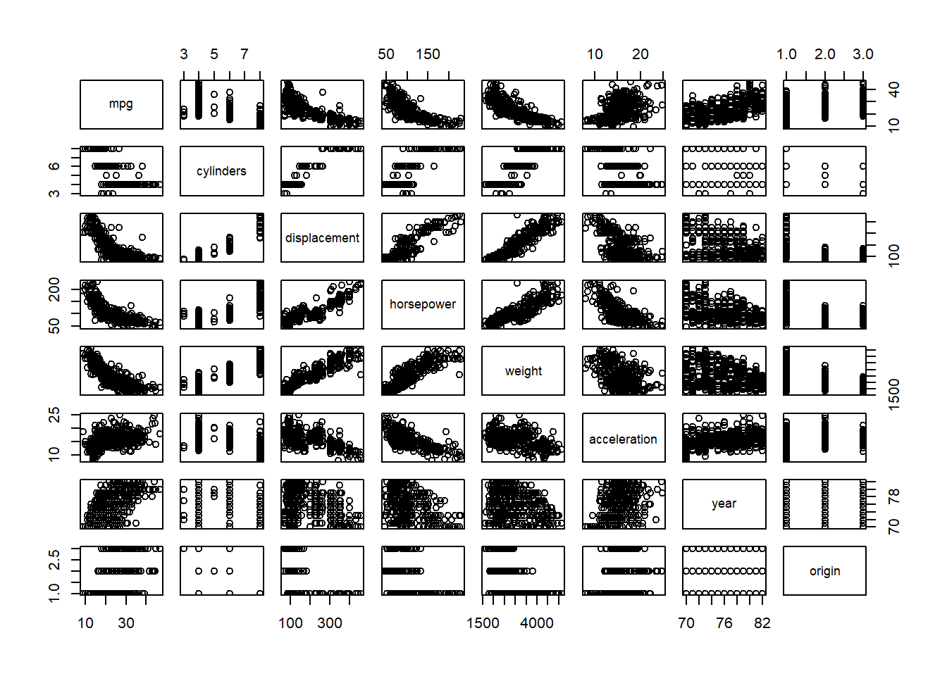
Briefly looking at the pairwise plots, the factors
cylinders,displacement,horsepower,weight, and possiblyyearare worth investigating.
library(ISLR2)
dim(Boston)
[1] 506 13506 rows each representing a town, 13 columns each with some data on the towns.
pairs(Boston)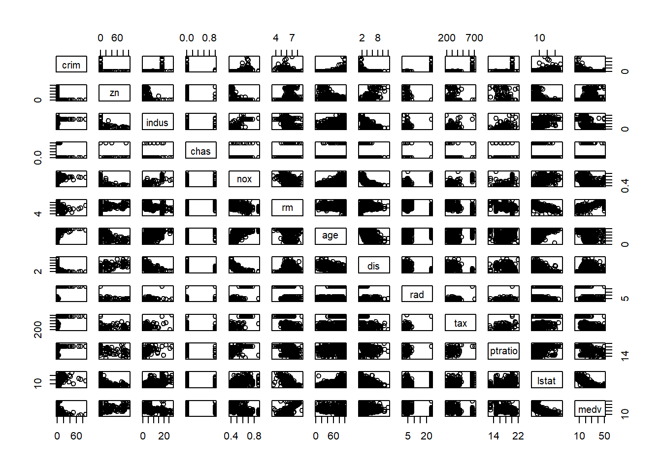
Various answers can exist:
crimrelates tozn,indus,age,dis,rad,tax,ptrationoxrelates toage,dis,radagerelates tolstat,medvlstatrelates tomedv
zn: Very low, unlessznis very close to 0. Thencrimcan be much higher.indus: Very low, unlessindusis close to 18%. Thencrimcan be much higher.age:crimincreases as this increasesdis:crimdecreases as this increasestax: Very low, unlesstaxis at 666ptratio: Very low, unlessptratiois at 20.2
par(mfrow = c(2, 2))
hist(Boston$crim, breaks = 25)
hist(Boston$tax)
hist(Boston$ptratio)
length(Boston$crim[Boston$crim > 20])
[1] 18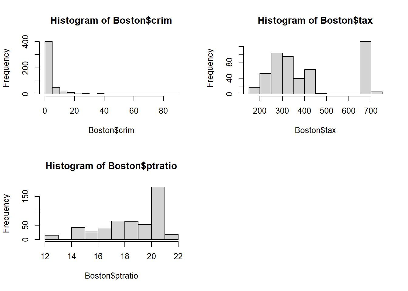
crim: Vast majority of cities have low crime rates, but 18 of them have a crime rate of greater than 20, reaching up to.tax: Divided into two sections: low < 500, high \ge 660.ptratio: Mode at about 20, max at 22, minimum at 12.6.
length(Boston$chas[Boston$chas == 1])[1] 35median(Boston$ptratio)[1] 19.05Boston[Boston$medv == min(Boston$medv), ]Crime rates are quite high,
indusis on the upper end, all owner-occupied units are built before 1940, both don’t bound the Charles river, both are relatively close to employment centres, they’re both very close to radial highways, pupil/teacher ratio is at the mode,lstatis also on the higher end.length(Boston$rm[Boston$rm > 7])[1] 64length(Boston$rm[Boston$rm > 8])[1] 13crim,lstatrelatively low.