Show the R package imports
library(caret)
library(ISLR2)
library(gbm)
library(maps)
library(rpart)
library(rpart.plot)
library(randomForest)
library(tidyverse)library(caret)
library(ISLR2)
library(gbm)
library(maps)
library(rpart)
library(rpart.plot)
library(randomForest)
library(tidyverse)import pandas as pd
import numpy as np
import matplotlib.pyplot as plt
from sklearn.tree import DecisionTreeRegressor
from sklearn.tree import plot_tree, export_textDecision trees
Bagging, random forests, boosting
Decision trees are a simple, easy to interpret, and popular method for both regression and classification tasks. They can be used to make predictions, but also simply as “data exploration” to understand a data set better.
They make predictions by partitioning the predictor space into a number of simple regions, and making a constant prediction within each region. The set of splitting rules can be summarised in a tree. “Stand alone” tree models are rarely particularly accurate, but they form the basis for more accurate (and complex) methods like random forests and boosting.

graph TB

    A{Is it peak hour?}
    A-->|Yes| B[Peak Hour]
    A-->|No| C[Off-Peak Hour]

    B--> D{Distance?}
    D-->|0 - 10 km| E[$3.79]
    D-->|10 - 20 km| F[$4.71]
    D-->|20 - 35 km| G[$5.42]
    D-->|35 - 65 km| H[$7.24]
    D-->|65+ km| I[$9.31]

    C--> J{Distance?}
    J-->|0 - 10 km| K[$2.65]
    J-->|10 - 20 km| L[$3.29]
    J-->|20 - 35 km| M[$3.79]
    J-->|35 - 65 km| N[$5.06]
    J-->|65+ km| O[$6.51]
rail_cost <- function(peak_hours, distance) {
  if (peak_hours) {
    if (distance <= 10) {
      cost <- 3.79
    } else if (distance <= 20) {
      cost <- 4.71
    } else if (distance <= 35) {
      cost <- 5.42
    } else if (distance <= 65) {
      cost <- 7.24
    } else {
      cost <- 9.31
    }
  } else {
    if (distance <= 10) {
      cost <- 2.65
    } else if (distance <= 20) {
      cost <- 3.29
    } else if (distance <= 35) {
      cost <- 3.79
    } else if (distance <= 65) {
      cost <- 5.06
    } else {
      cost <- 6.51
    }
  }
  return(cost)
}
def rail_cost(peak_hours, distance):
if peak_hours:
if distance <= 10:
cost = 3.79
elif distance <= 20:
cost = 4.71
elif distance <= 35:
cost = 5.42
elif distance <= 65:
cost = 7.24
else:
cost = 9.31
else:
if distance <= 10:
cost = 2.65
elif distance <= 20:
cost = 3.29
elif distance <= 35:
cost = 3.79
elif distance <= 65:
cost = 5.06
else:
cost = 6.51
return costHitters datasetdata(Hitters)
Hittershitters = pd.read_csv('Hitters.csv')
hitters Unnamed: 0 AtBat Hits HmRun ... Assists Errors Salary NewLeague
0 -Alan Ashby 315 81 7 ... 43 10 475.0 N
1 -Alvin Davis 479 130 18 ... 82 14 480.0 A
2 -Andre Dawson 496 141 20 ... 11 3 500.0 N
3 -Andres Galarraga 321 87 10 ... 40 4 91.5 N
4 -Alfredo Griffin 594 169 4 ... 421 25 750.0 A
.. ... ... ... ... ... ... ... ... ...
258 -Willie McGee 497 127 7 ... 9 3 700.0 N
259 -Willie Randolph 492 136 5 ... 381 20 875.0 A
260 -Wayne Tolleson 475 126 3 ... 113 7 385.0 A
261 -Willie Upshaw 573 144 9 ... 131 12 960.0 A
262 -Willie Wilson 631 170 9 ... 4 3 1000.0 A
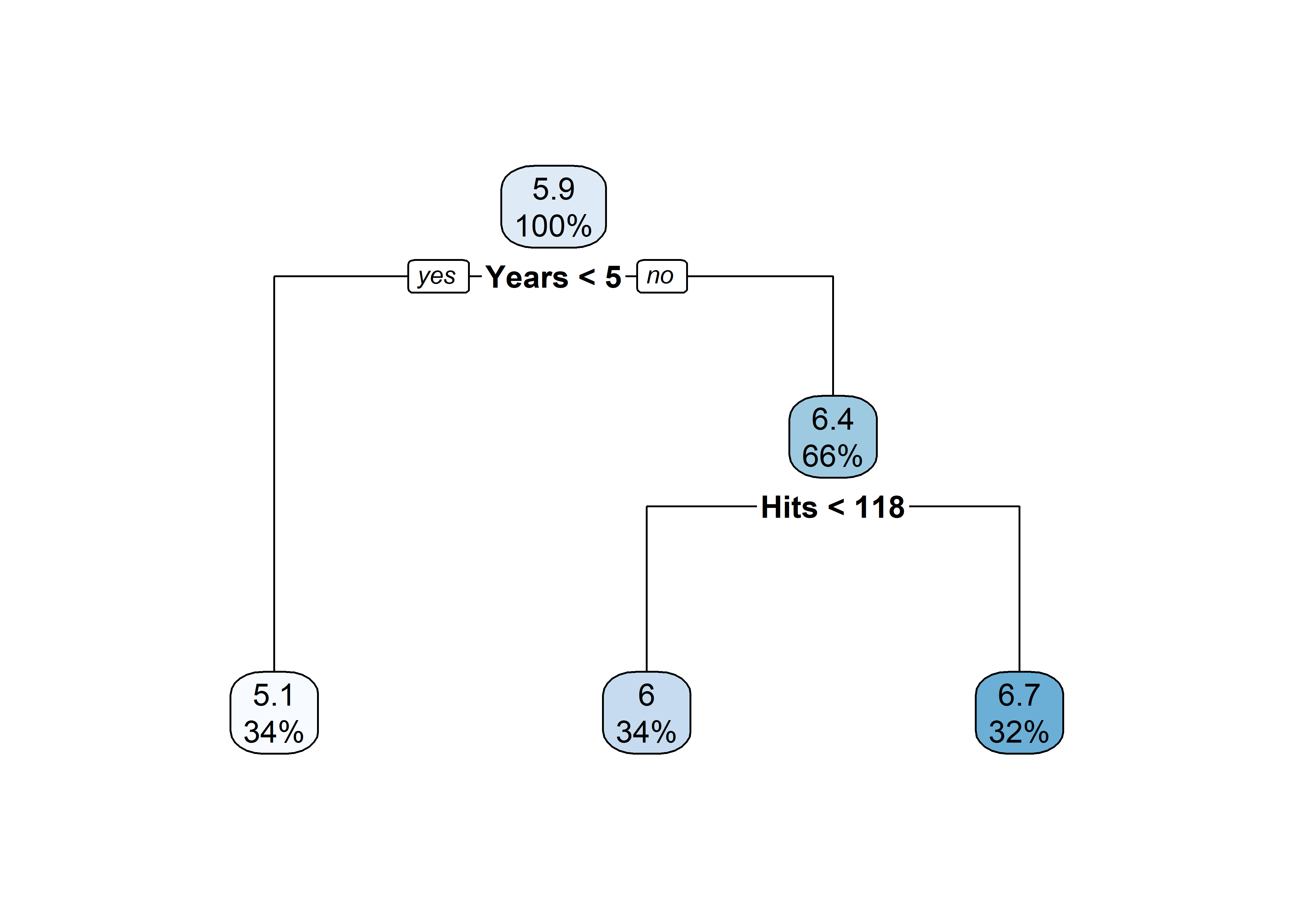
[263 rows x 21 columns](tree <- rpart(
log(Salary) ~ Years + Hits,
data = Hitters))n= 263
node), split, n, deviance, yval
* denotes terminal node
1) root 263 207.153700 5.927222
2) Years< 4.5 90 42.353170 5.106790
4) Years< 3.5 62 23.008670 4.891812
8) Hits< 114 43 17.145680 4.727386 *
9) Hits>=114 19 2.069451 5.263932 *
5) Years>=3.5 28 10.134390 5.582812 *
3) Years>=4.5 173 72.705310 6.354036
6) Hits< 117.5 90 28.093710 5.998380
12) Years< 6.5 26 7.237690 5.688925 *
13) Years>=6.5 64 17.354710 6.124096
26) Hits< 50.5 12 2.689439 5.730017 *
27) Hits>=50.5 52 12.371640 6.215037 *
7) Hits>=117.5 83 20.883070 6.739687 *plot(tree)
text(tree)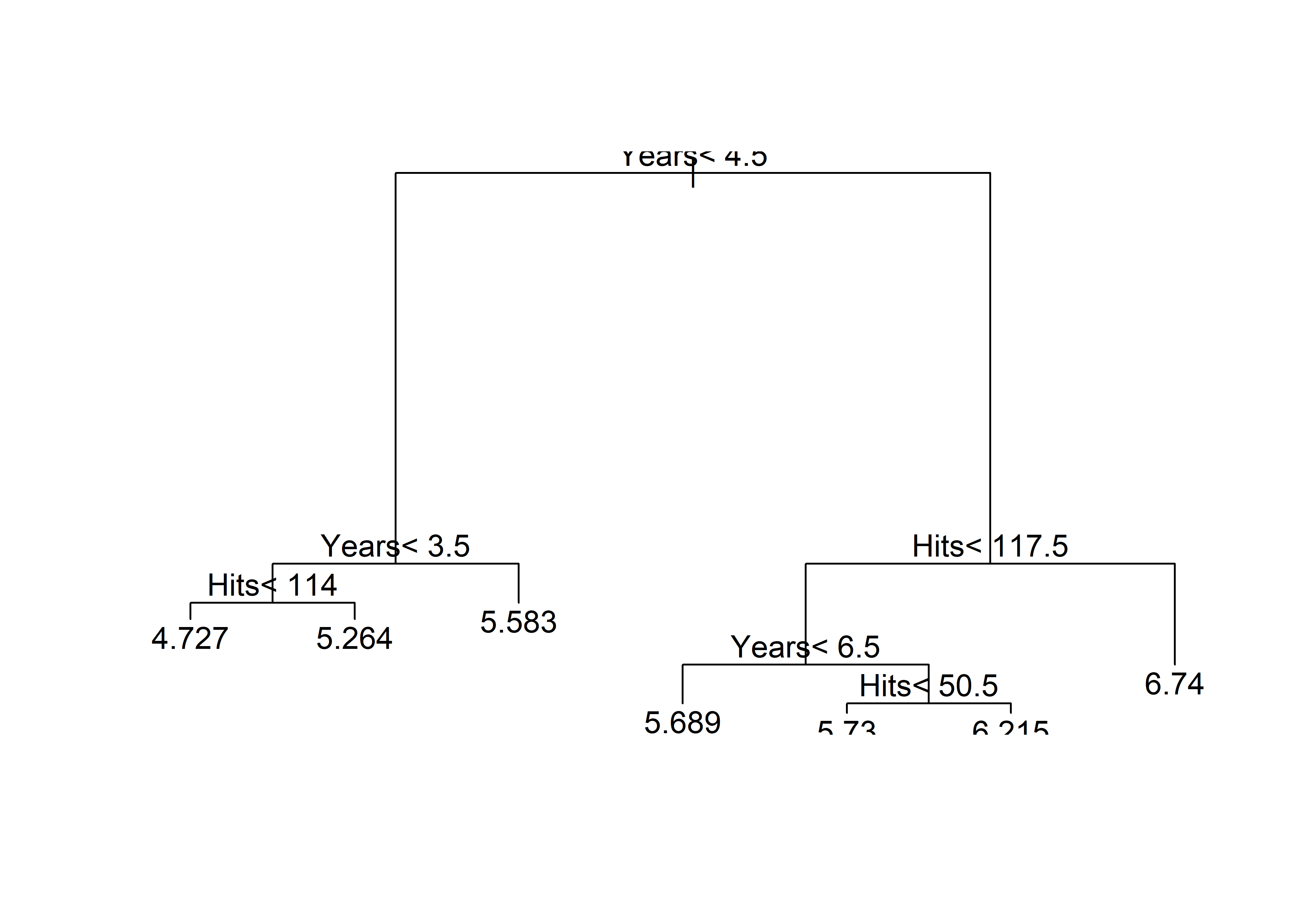
X = hitters[['Years', 'Hits']]
y = np.log(hitters['Salary'])
tree = DecisionTreeRegressor(min_samples_split=20, min_samples_leaf=10, max_depth=3, ccp_alpha=0.01)
tree.fit(X, y);
print(export_text(tree, feature_names=['Years', 'Hits']))
|--- Years <= 4.50
| |--- Years <= 3.50
| | |--- Hits <= 114.00
| | | |--- value: [4.73]
| | |--- Hits > 114.00
| | | |--- value: [5.26]
| |--- Years > 3.50
| | |--- value: [5.58]
|--- Years > 4.50
| |--- Hits <= 117.50
| | |--- Years <= 6.50
| | | |--- value: [5.69]
| | |--- Years > 6.50
| | | |--- value: [6.12]
| |--- Hits > 117.50
| | |--- value: [6.74]rpart.plot(tree)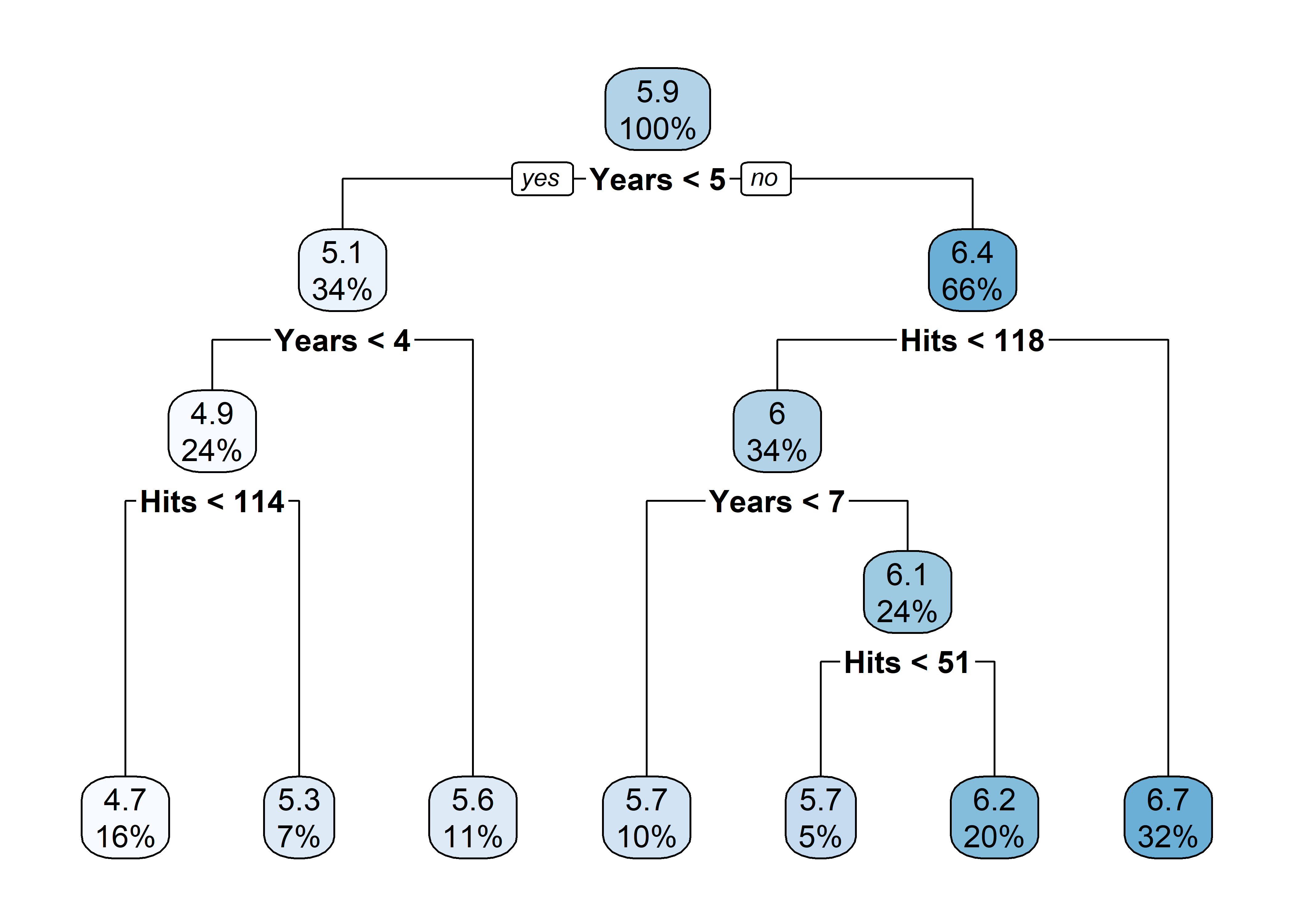
plot_tree(tree, feature_names = ['Years', 'Hits'], filled = True, rounded = True, impurity = False, proportion = True)
plt.show()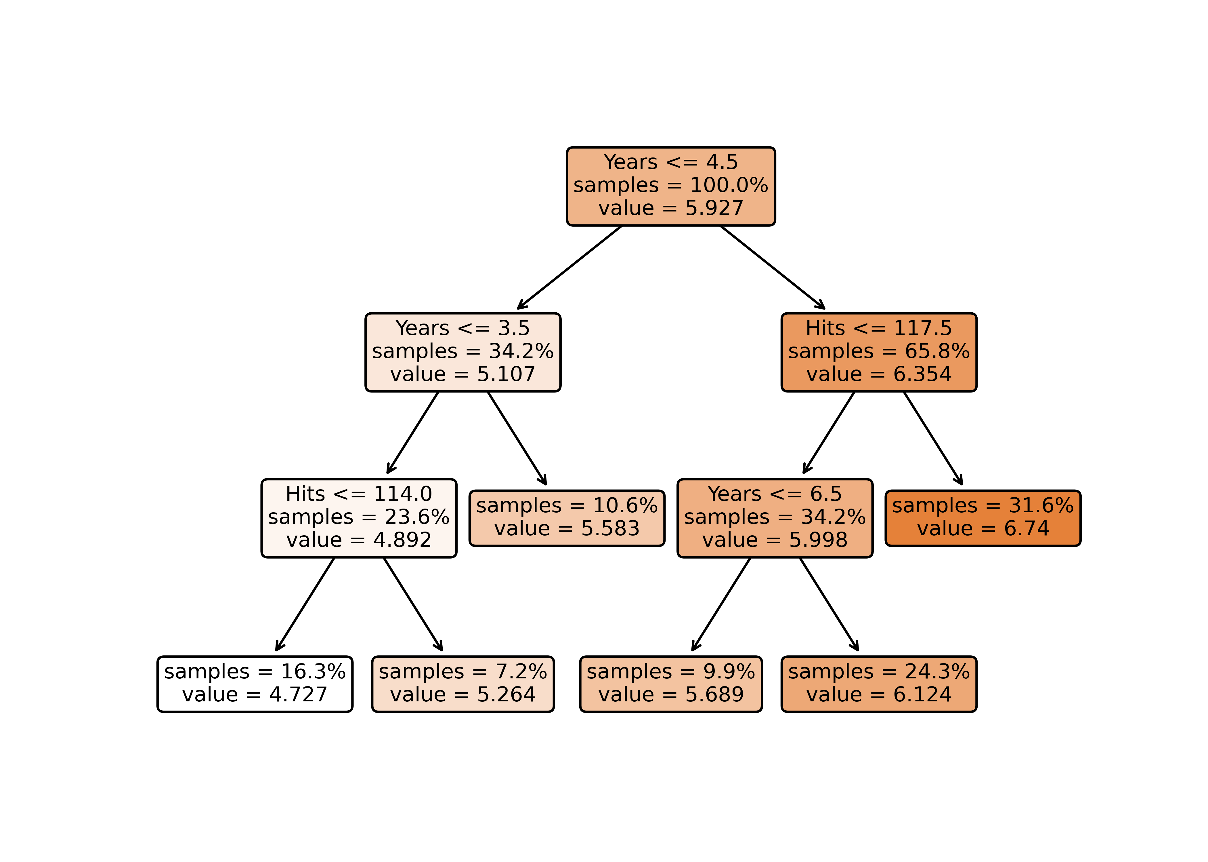
pruned_tree <- prune(tree, cp = tree$cptable[3, "CP"])
rpart.plot(pruned_tree)
rpart.plot(pruned_tree)
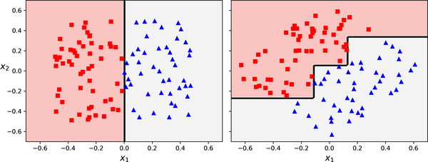
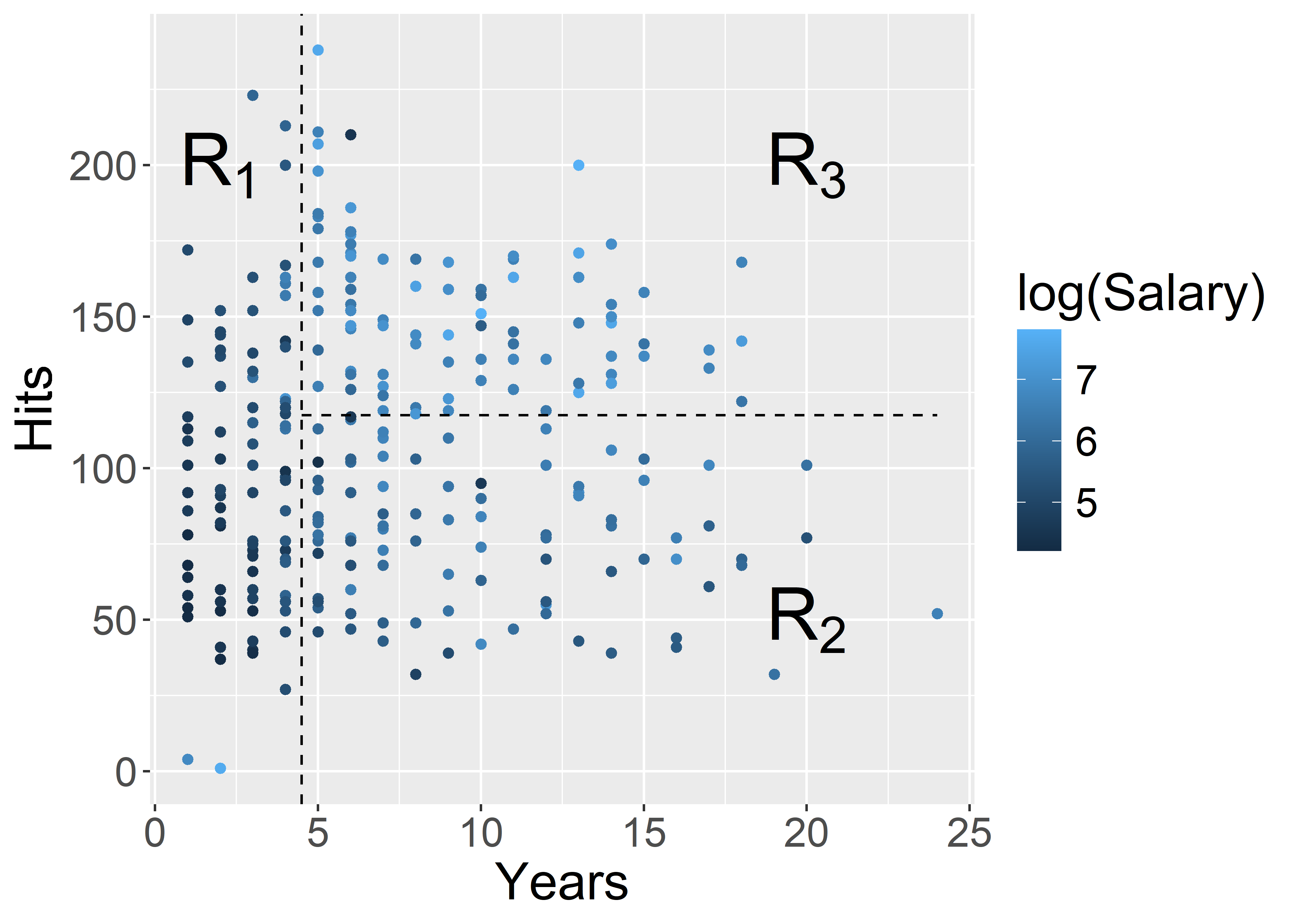
ggplot(Hitters, aes(x = Years, y = Hits, colour = log(Salary))) +
  geom_point() +
  geom_vline(xintercept = 4.5, colour = "black", linetype = "dashed") +
  annotate("segment", x = 4.5, xend = 24, y = 117.5, yend = 117.5, colour = "black", linetype = "dashed") +
  annotate("text", x = 2, y = 200, label = "R[1]", parse = TRUE, size = 10) +
  annotate("text", x = 20, y = 50, label = "R[2]", parse = TRUE, size = 10) +
  annotate("text", x = 20, y = 200, label = "R[3]", parse = TRUE, size = 10) +
  theme(text = element_text(size = 20))
A decision tree is made by:
Hitters example:
| Region | Predicted salaries |
|---|---|
| R_1 = \{X | \mathtt{Years} < 4.5 \} | \$1,000 \times \mathrm{e}^{5.107} = \$165,174 |
| R_2 = \{X | \mathtt{Years} \geq 4.5, \mathtt{Hits} < 117.5 \} | \$1,000 \times \mathrm{e}^{5.999} = \$402,834 |
| R_3 = \{X | \mathtt{Years} \geq 4.5, \mathtt{Hits} \geq 117.5 \} | \$1,000 \times \mathrm{e}^{6.740} = \$845,346 |
How do you interpret the results of this tree? In particular, consider the following questions
Salary?Hits affect Salary?rpart.plot(pruned_tree)

A decision tree enforces binary splits…
graph TB

    A{Peak hour?}
    A-->|Yes| B[Peak Hour]
    A-->|No| C[Off-Peak Hour]

    B--> D{Distance?}
    D-->|0 - 10 km| E[$3.79]
    D-->|10 - 20 km| F[$4.71]
    D-->|20 - 35 km| G[$5.42]
    D-->|35 - 65 km| H[$7.24]
    D-->|65+ km| I[$9.31]

    C--> J{Distance?}
    J-->|0 - 10 km| K[$2.65]
    J-->|10 - 20 km| L[$3.29]
    J-->|20 - 35 km| M[$3.79]
    J-->|35 - 65 km| N[$5.06]
    J-->|65+ km| O[$6.51]
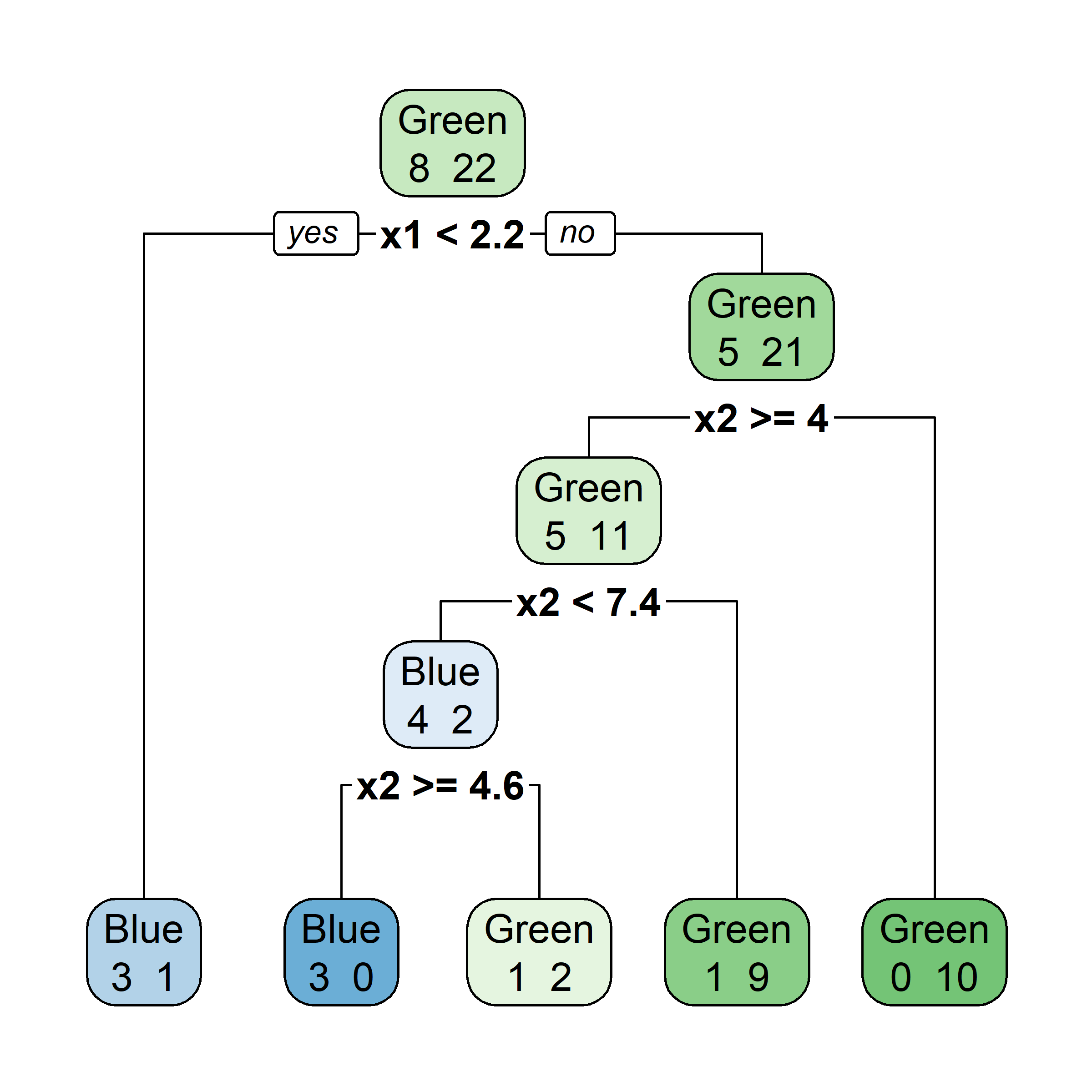
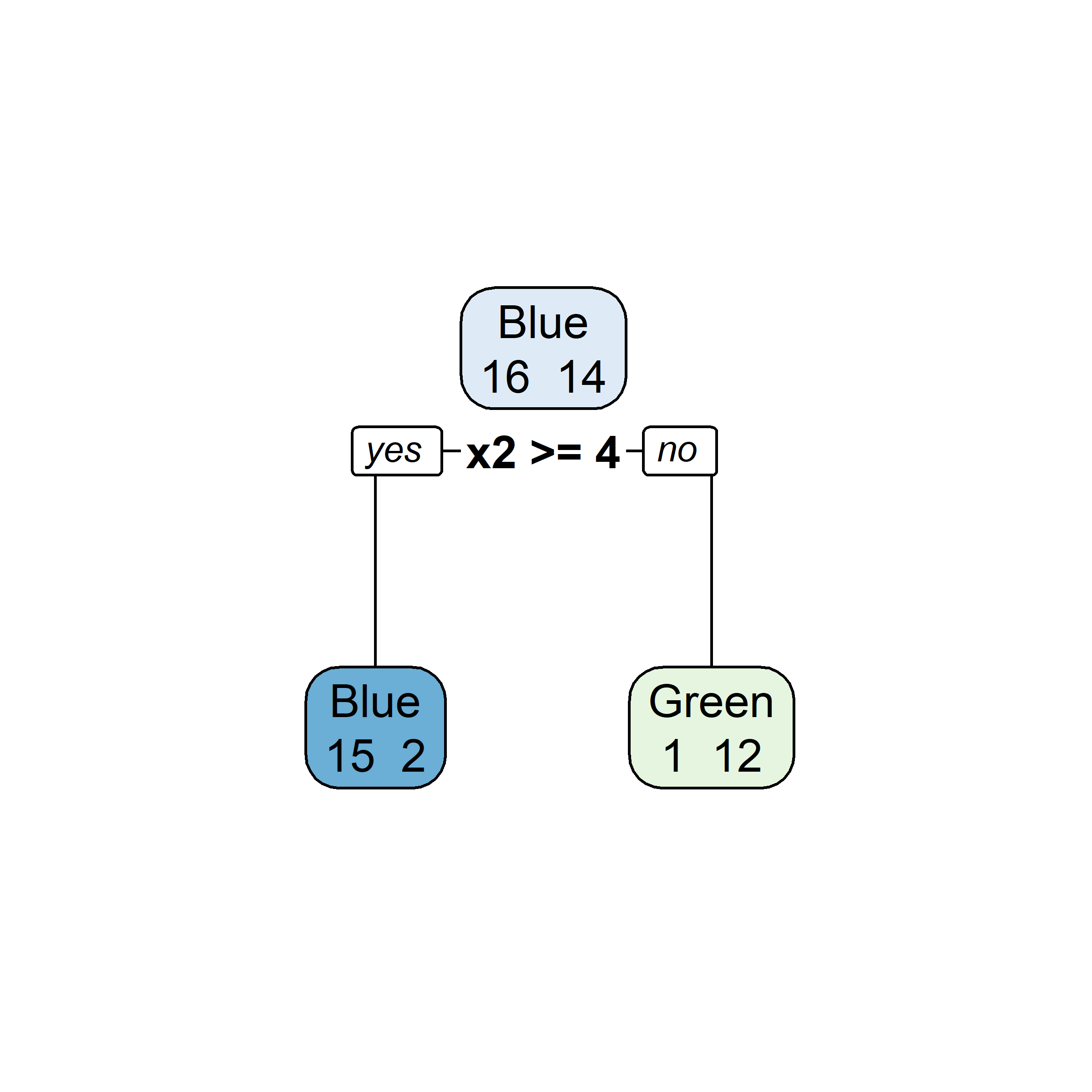
… but we can still represent non-binary splits in a binary tree.
graph TB
    A{Peak hour?}
    A-->|Yes| B[Peak Hour]
    A-->|No| J[Off-Peak Hour]

    B--> D1[0 - 10 km: $3.79]
    B--> D2[10 km +]
    D2--> F1[10 - 20 km: $4.71]
    D2--> G1[20 km +]
    G1--> H1[20 - 35 km: $5.42]
    G1--> I1[35 km +]
    I1--> I2[35 - 65 km: $7.24]
    I1--> I3[65 km +: $9.31]

    J--> K1[0 - 10 km: $2.65]
    J--> L1[10 km +]
    L1--> L2[10 - 20 km: $3.29]
    L1--> M1[20 km +]
    M1--> M2[20 - 35 km: $3.79]
    M1--> N1[35 km +]
    N1--> N2[35 - 65 km: $5.06]
    N1--> O[65 km +: $6.51]


Consider a splitting variable j and split point s R_1(j, s) = \{X | X_j \leq s\} \quad \text{and} \quad R_2(j, s) = \{X|X_j>s\}
Find the splitting variable j and split point s that solve \min_{j,\ s}\Big[ \min_{c_1} \sum_{x_i \in R_1(j,\ s)}(y_i-c_1)^2 + \min_{c_2} \sum_{x_i \in R_2(j,\ s)}(y_i-c_2)^2 \Big] where the inner mins are solved by \hat{c}_1 = \mathrm{Ave}(y_i | x_i \in R_1(j, s)) \quad \text{and} \quad \hat{c}_2 = \mathrm{Ave}(y_i | x_i \in R_2(j, s))
After this first split, “we repeat the process, looking for the best predictor and best cutpoint in order to split the data further so as to minimize the RSS within each of the resulting regions. However, this time, instead of splitting the entire predictor space, we split one of the two previously identified regions.” (James et al., 2021)
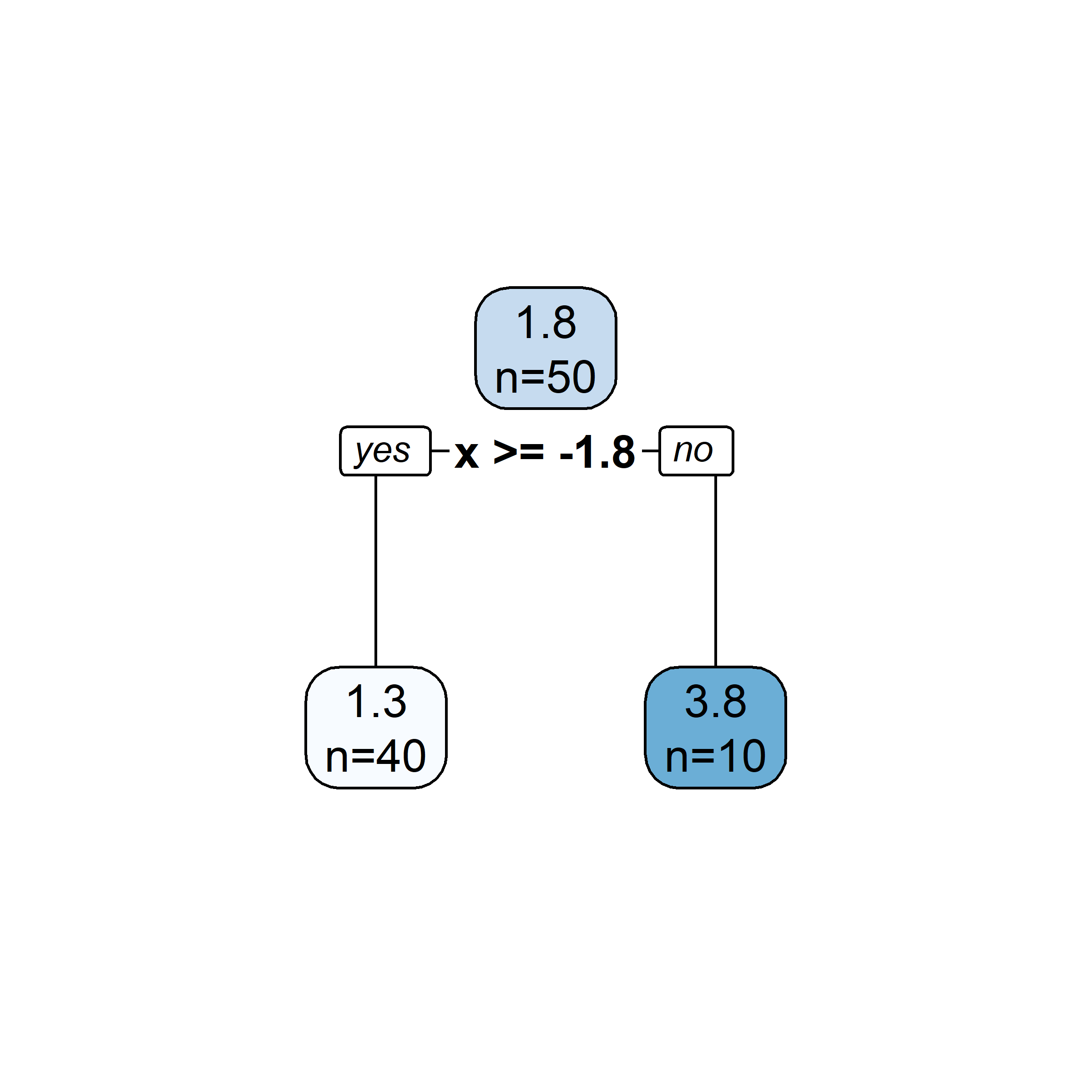
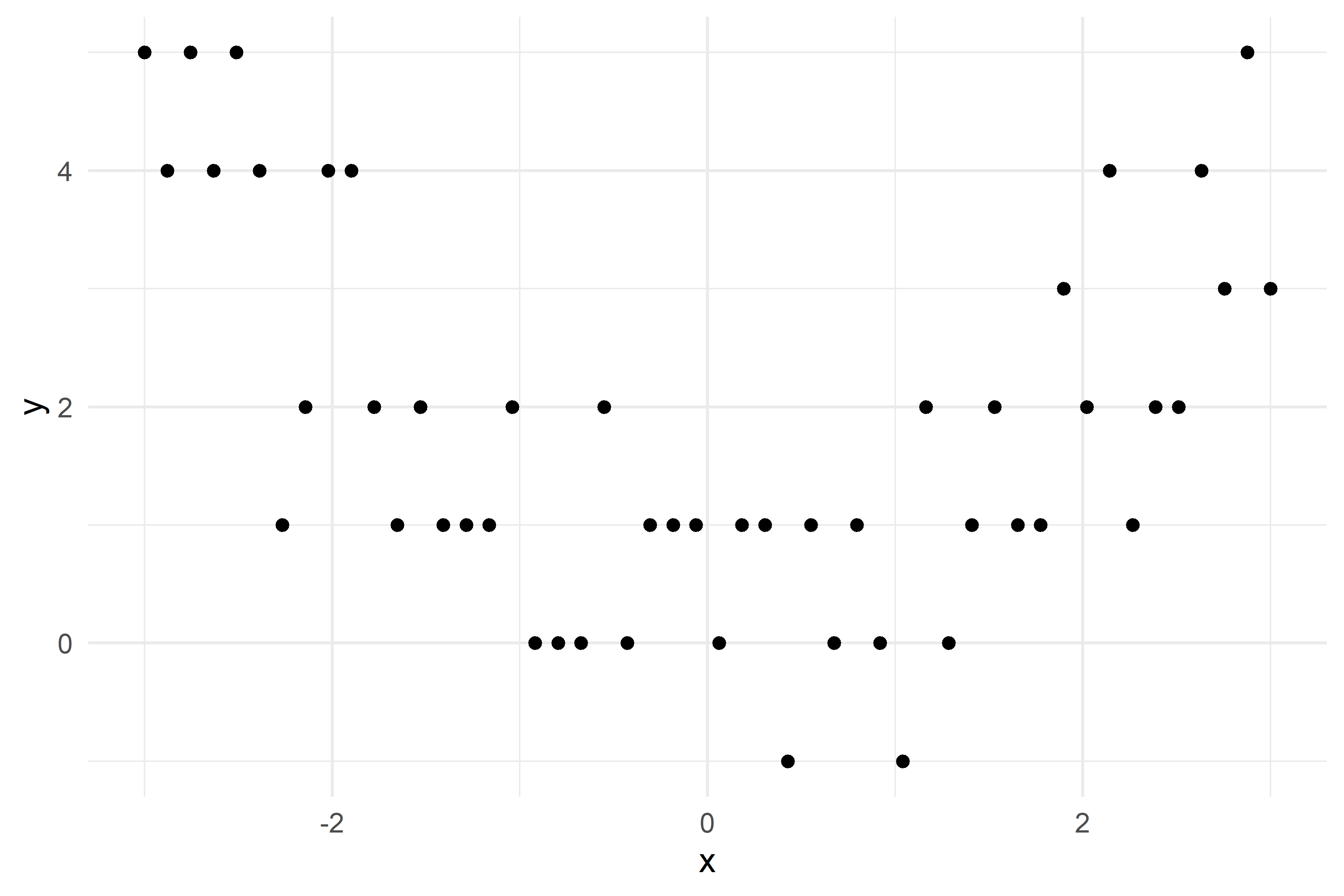
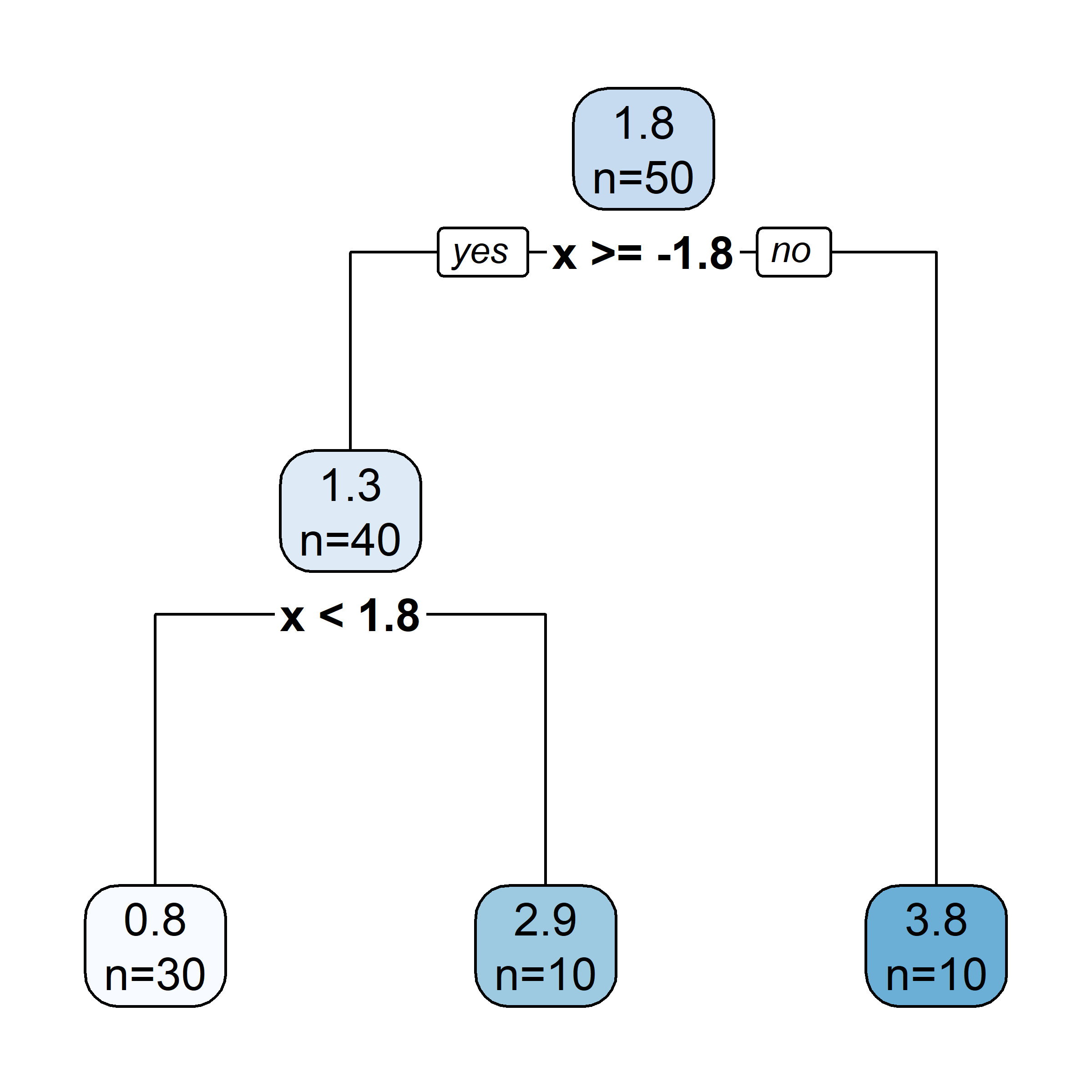
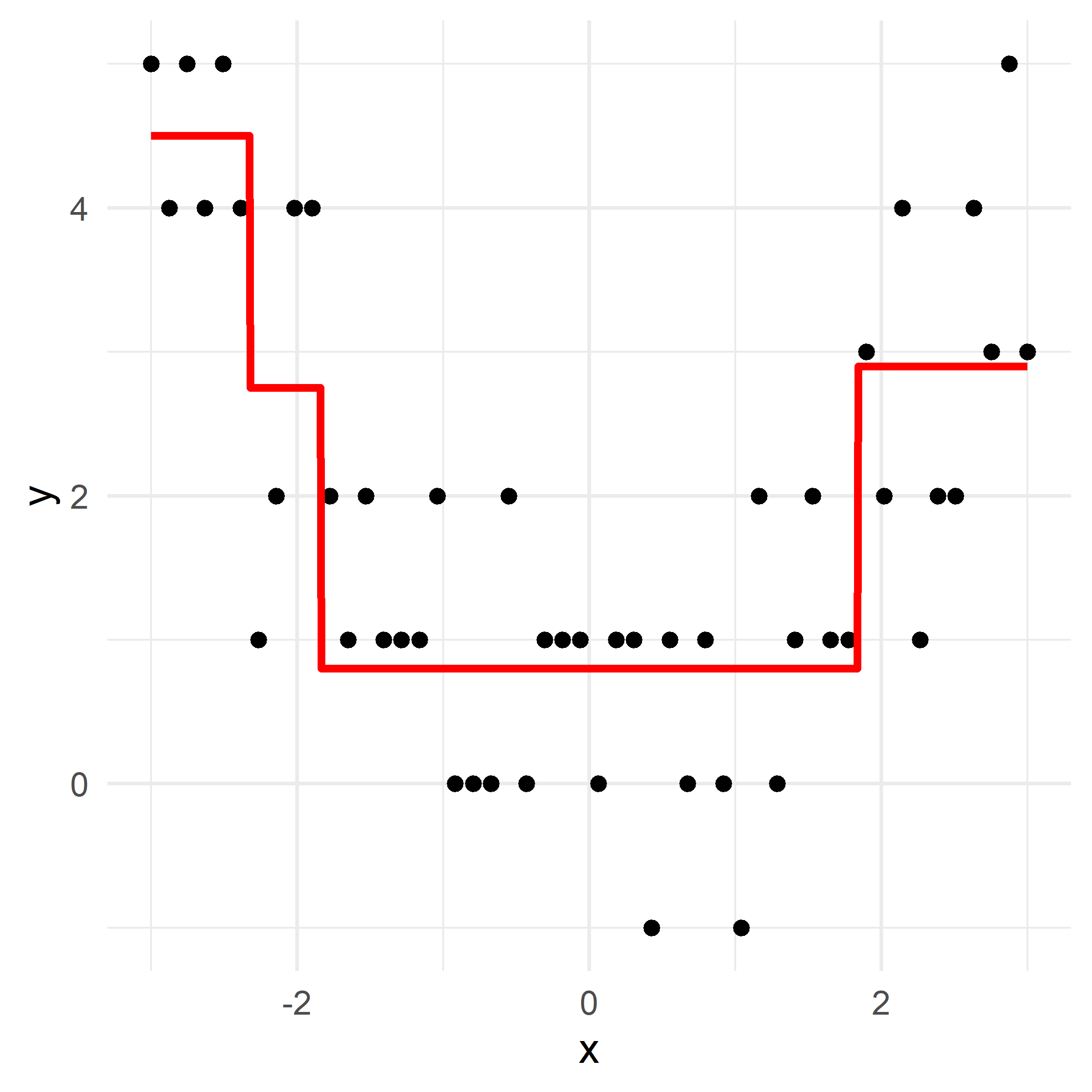
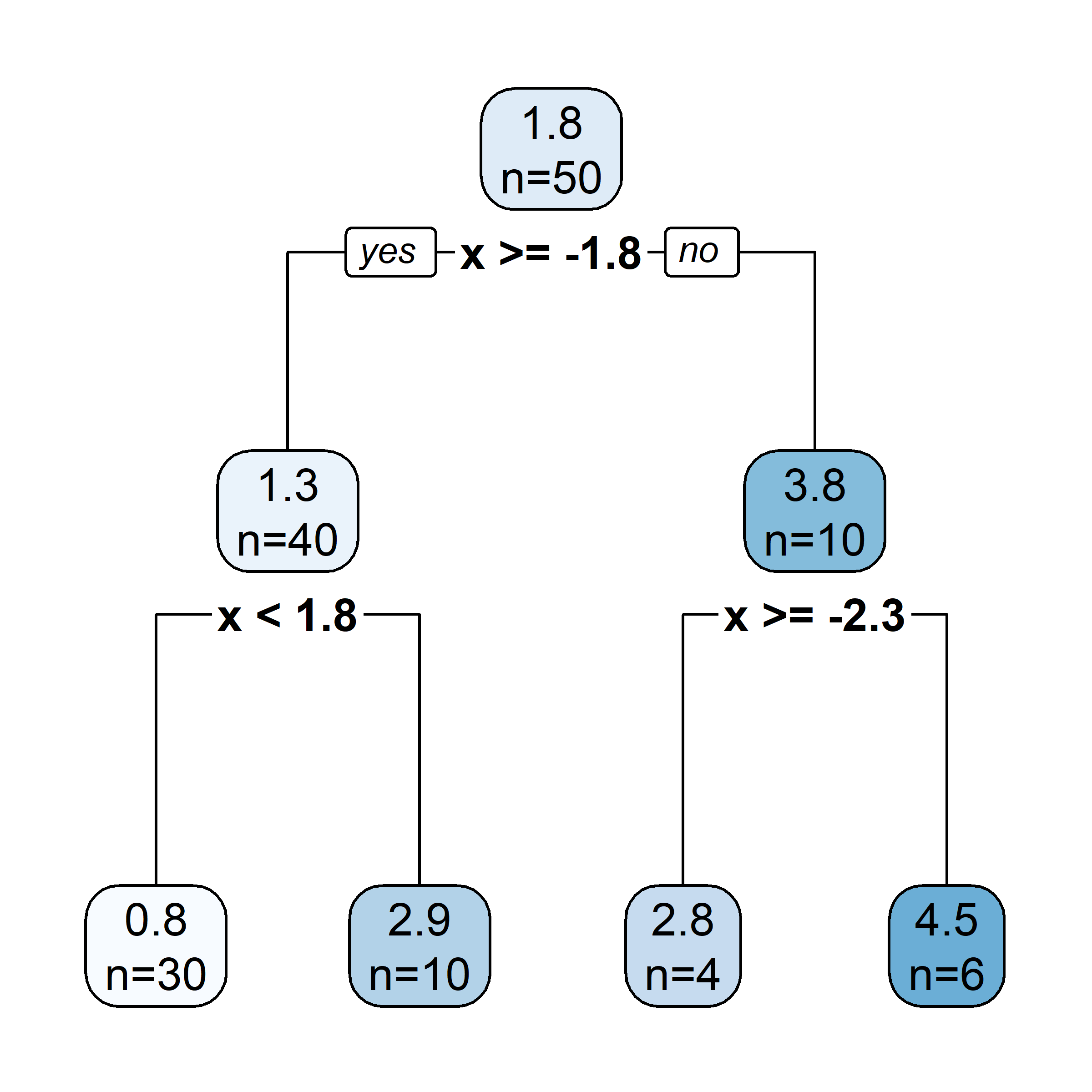
What would be the tree’s predicted value for y at x = 0?
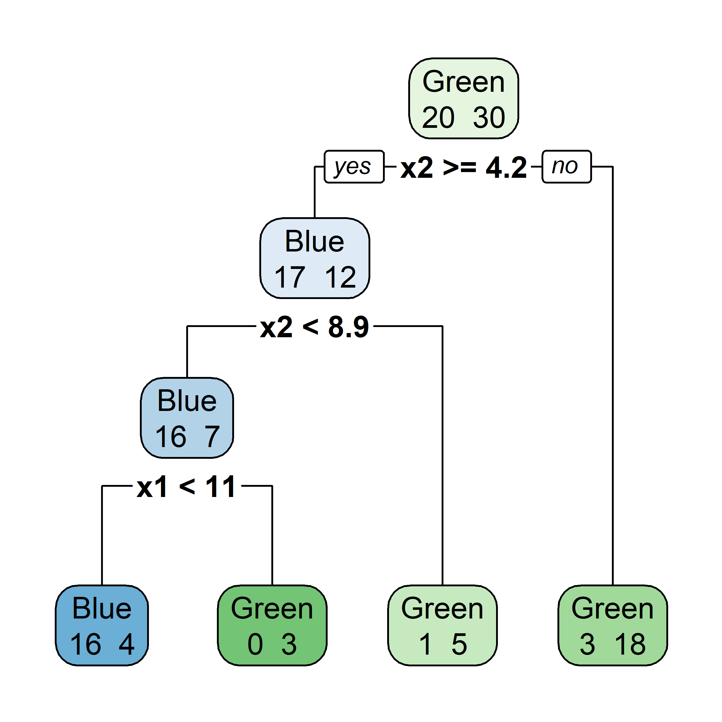
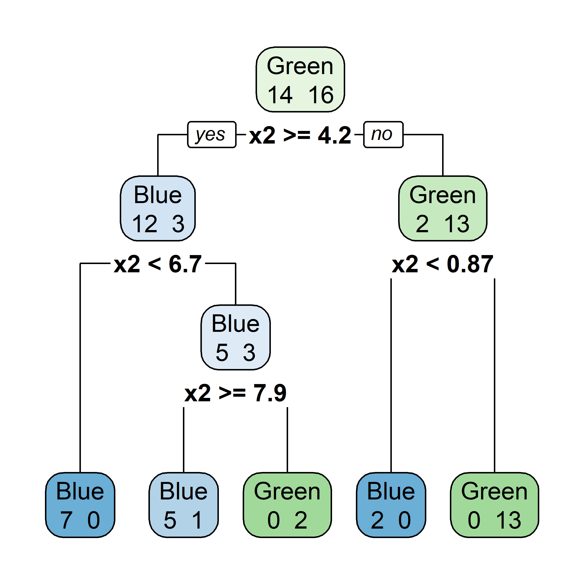
Very similar to a regression tree, except:
Gini index, or
G = \sum_{k=1}^{K}\hat{p}_{mk}(1 - \hat{p}_{mk})
entropy
D = -\sum_{k=1}^{K}\hat{p}_{mk}\ln(\hat{p}_{mk})
where \hat{p}_{mk} = \frac{1}{| R_m | }\sum_{x_i \in R_m}I(y_i = k) \,.


rpart.plot(tree4, type = 0)
rpart.plot(tree4, type = 2)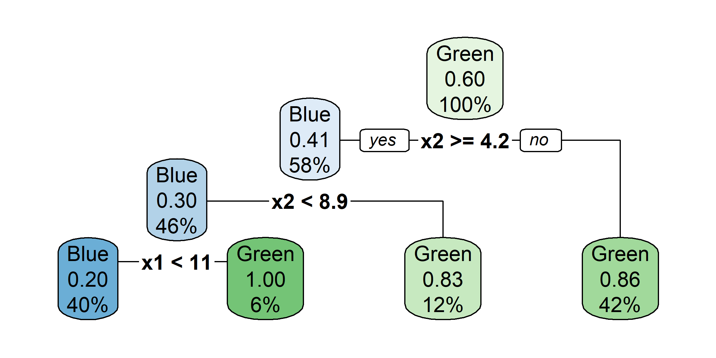
rpart.plot(tree4, type = 3)
rpart.plot(tree4, type = 5)
rpart.plot(tree4, type = 1, extra = 2)
rpart.plot(tree4, type = 1, extra = 4)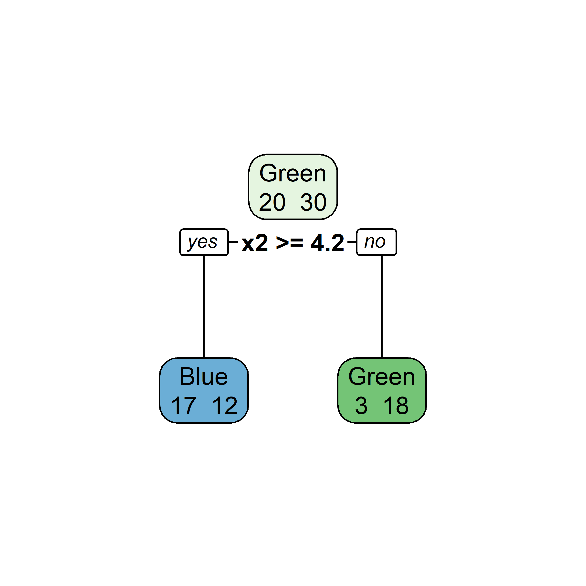
rpart.plot(tree4, type = 1, extra = 3)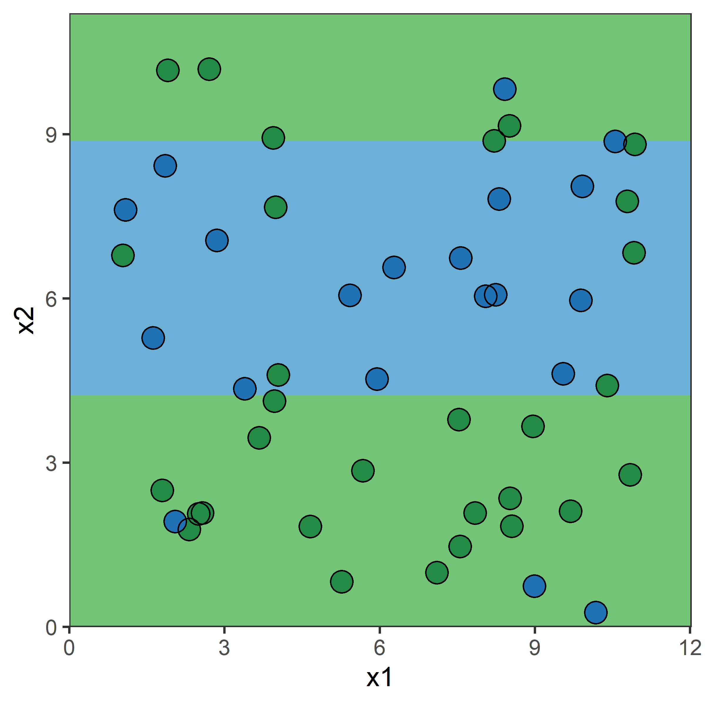
rpart.plot(tree4, type = 1, extra = 5)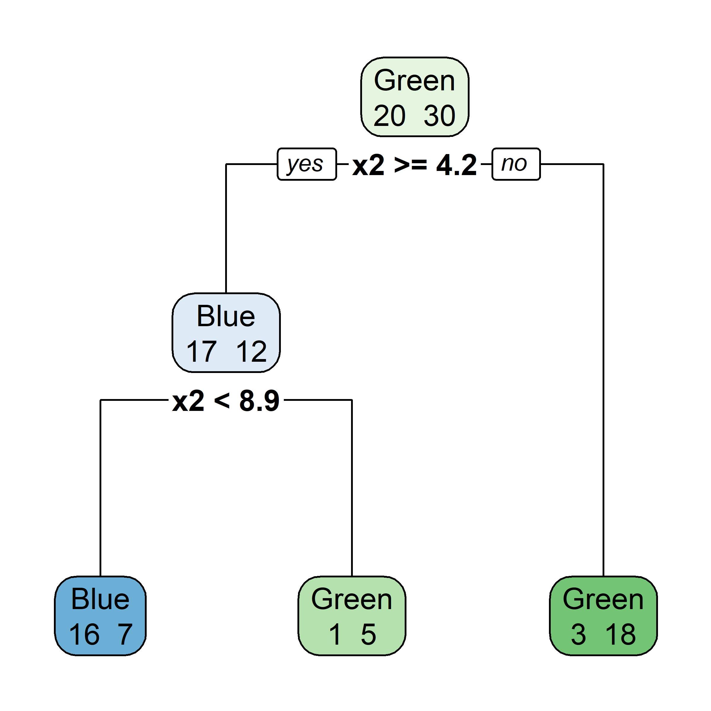
So, should you use Gini impurity or entropy? The truth is, most of the time it does not make a big difference: they lead to similar trees. Gini impurity is slightly faster to compute, so it is a good default. However, when they differ, Gini impurity tends to isolate the most frequent class in its own branch of the tree, while entropy tends to produce slightly more balanced trees.
See also Sebastian Raschka’s interesting analysis for more details.
Available at OpenFEMA dataset.
claims <- read.csv("FimaNfipClaimsClean.csv")
| Name | Title | Type | Description |
|---|---|---|---|
| id | ID | text | Unique ID assigned to the record |
| amountPaidOnBuildingClaim | Amount Paid on Building Claim | decimal | Dollar amount paid on the building claim. In some instances, a negative amount may appear. |
| agricultureStructureIndicator | Agriculture Structure Indicator | boolean | Indicates whether a building is reported as being an agricultural structure in the policy application. |
| policyCount | Policy Count | smallint | Insured units in an active status. A policy contract ceases to be in an active status as of the cancellation date or the expiration date. |
| countyCode | County Code | text | FIPS code uniquely identifying the primary County (e.g., 011 represents Broward County) associated with the project. |
| lossDate | Date of Loss | datetime | Date on which water first entered the insured building. |
| elevatedBuildingIndicator | Elevated Building Indicator | boolean | Indicates whether a building meets the NFIP definition of an elevated building. |
| latitude | Latitude | decimal | Approximate latitude of the insured building. |
| locationOfContents | Location of Contents | smallint | Code that indicates the location of contents, (e.g., garage on property, in house). |
| Name | Title | Type | Description |
|---|---|---|---|
| longitude | Longitude | decimal | Approximate longitude of the insured building. |
| lowestFloorElevation | Lowest Floor Elevation | decimal | A building’s lowest floor is the floor or level that is used as the point of reference when rating a building. |
| numberOfFloors | Number of Floors | smallint | Code that indicates the number of floors in the insured building. |
| occupancyType | Occupancy Type | smallint | Code indicating the use and occupancy type of the insured structure. |
| originalConstructionDate | Original Construction Date | date | The original date of the construction of the building. |
| originalNBDate | Original NB Date | date | The original date of the flood policy. |
| postFIRMConstructionIndicator | Post-FIRM Construction Indicator | boolean | Indicates whether construction was started before or after publication of the FIRM. |
| rateMethod | Rate Method | text | Indicates policy rating method. |
| state | State | text | The two-character alpha abbreviation of the state in which the insured property is located. |
| totalBuildingInsuranceCoverage | Total Building Insurance Coverage | integer | Total Insurance Amount in whole dollars on the Building. |
tree <- rpart(amountPaidOnBuildingClaim ~ ., data=claims[1:1000,])
rpart.plot(tree)
Warning: labs do not fit even at cex 0.15, there may be some overplotting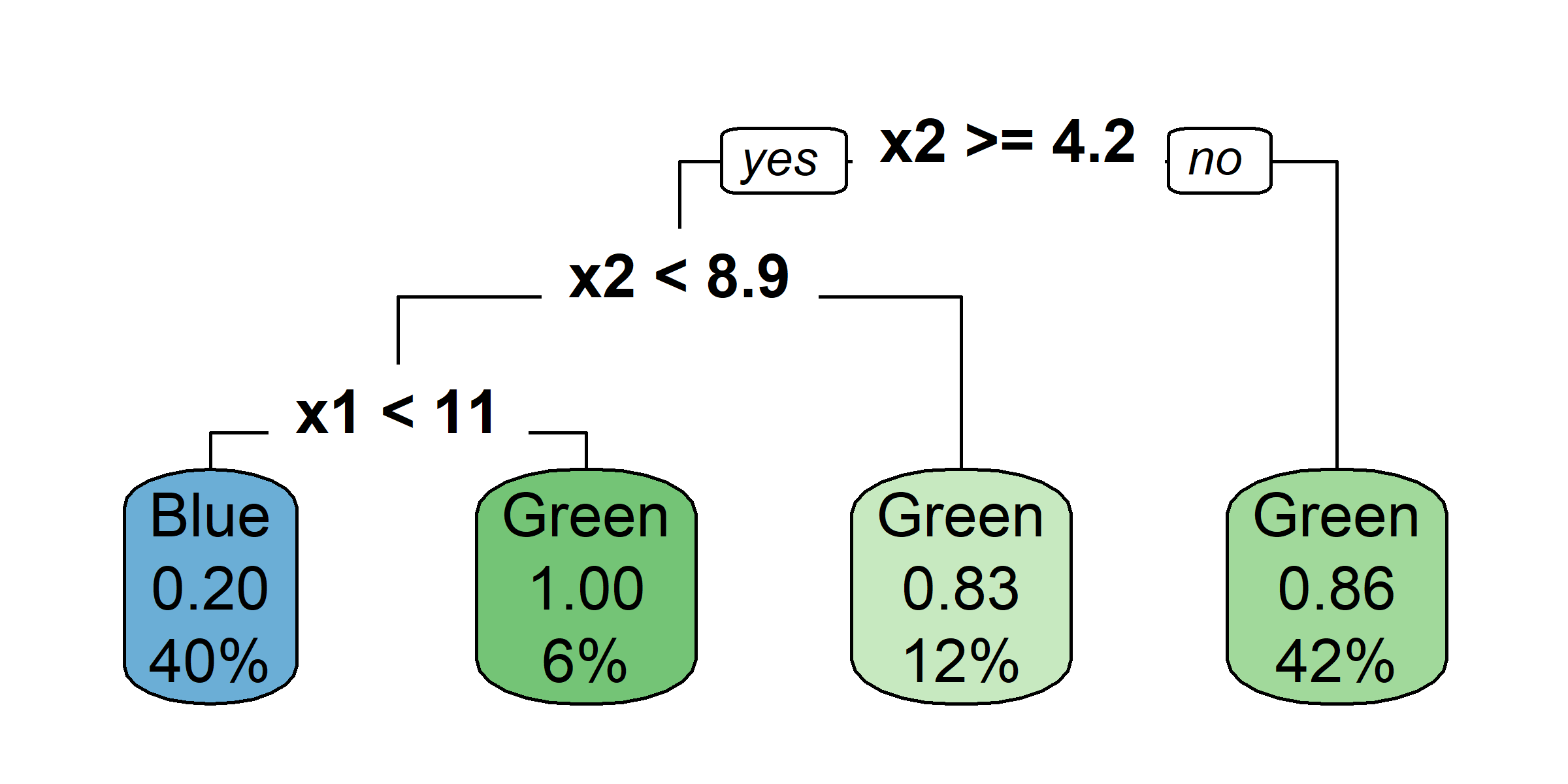
claims <- claims %>% select(-id)
tree <- rpart(amountPaidOnBuildingClaim ~ ., data=claims[1:1000,])
rpart.plot(tree)
claims$lossYear <- year(claims$lossDate) # And so on...claims$lossYear <- year(claims$lossDate)
claims$lossMonth <- month(claims$lossDate)
claims$lossDate <- NULL
claims$originalConstructionYear <- year(claims$originalConstructionDate)
claims$originalConstructionMonth <- month(claims$originalConstructionDate)
claims$originalConstructionDate <- NULL
claims$originalNBYear <- year(claims$originalNBDate)
claims$originalNBMonth <- month(claims$originalNBDate)
claims$originalNBDate <- NULLtree <- rpart(amountPaidOnBuildingClaim ~ ., data=claims[1:1000,])
rpart.plot(tree)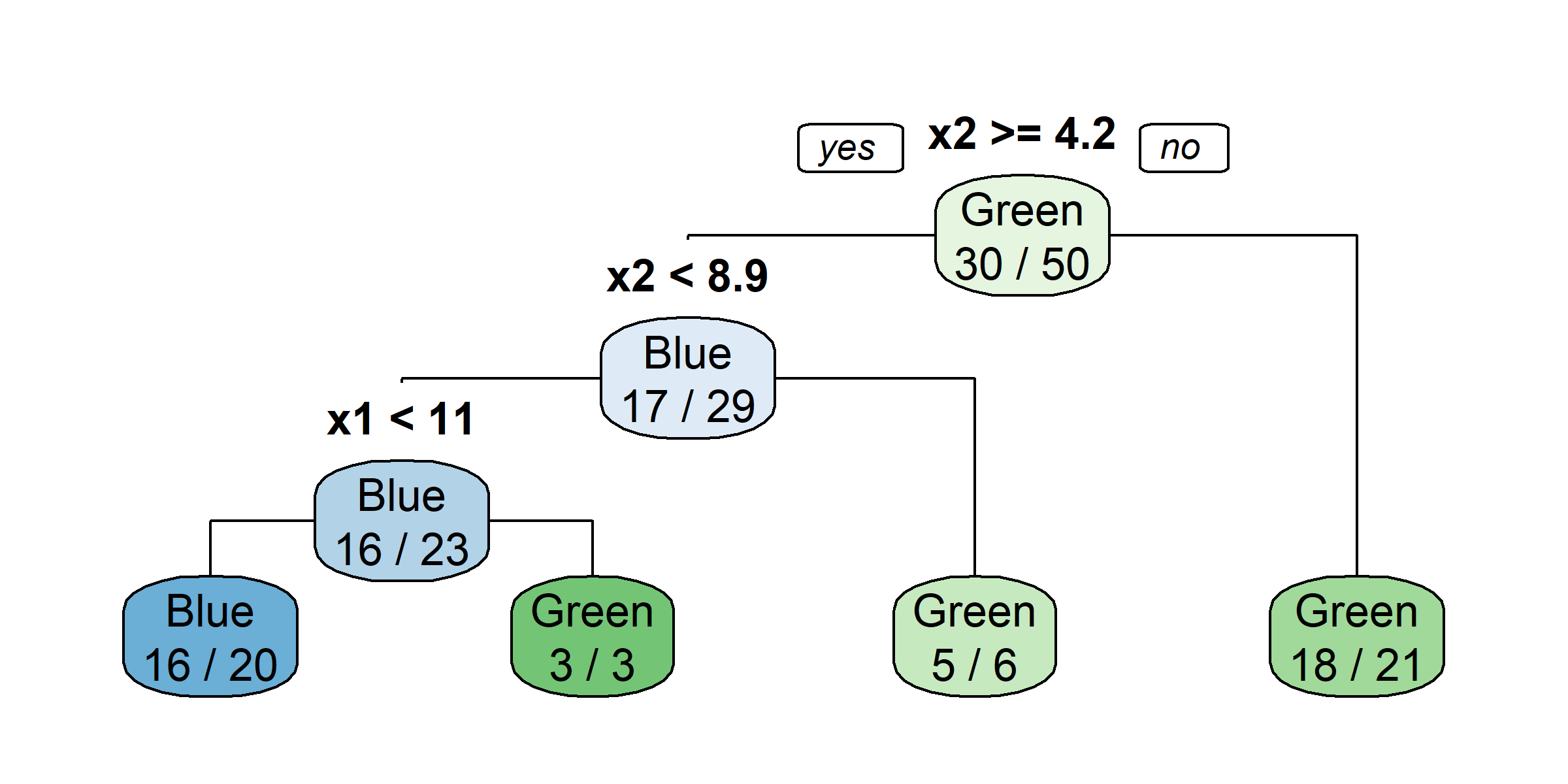
claims %>%
  group_by(lossYear) %>%
  summarise(n = n()) %>%
  ggplot(aes(x = lossYear, y = n)) +
  geom_bar(stat = "identity") +
  theme_minimal() +
  labs(x = "Year", y = "Number of claims")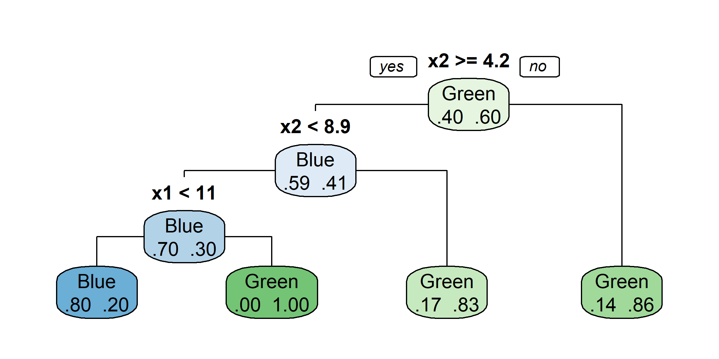
claims %>%
  group_by(lossYear) %>%
  summarise(mean_claim = mean(amountPaidOnBuildingClaim)) %>%
  ggplot(aes(x = lossYear, y = mean_claim)) +
  geom_line() +
  theme_minimal() +
  labs(x = "Year", y = "Average claim size")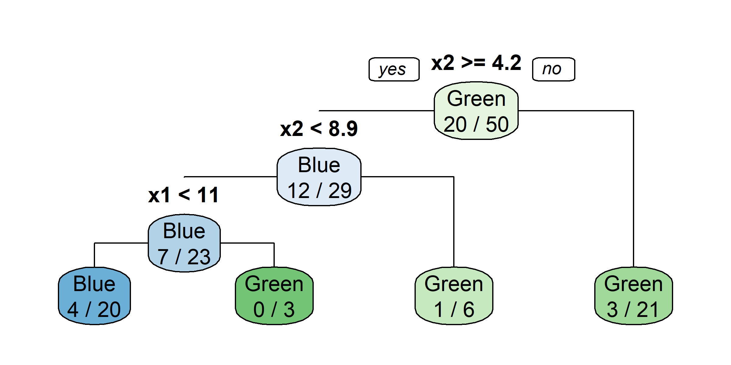
claims$state_full <- state.name[match(claims$state, state.abb)]

state_claims <- claims %>%
  group_by(state_full) %>%
  summarise(num_claims = n(),
            max_claim_size = max(amountPaidOnBuildingClaim),
            common = num_claims >= nrow(claims) / 100)

claims$state_full <- NULL

# Merge with the map data
states_map <- map_data("state")
state_claims$region <- tolower(state_claims$state_full)
states_map <- left_join(states_map, state_claims, by = "region")ggplot(states_map, aes(long, lat, group = group, fill = num_claims)) +
geom_polygon(color = "white") +
scale_fill_viridis_c(option = "C") +
labs(title = "Number of Claims by State",
fill = "Number of Claims") +
theme_minimal() +
theme(axis.title = element_blank(), axis.text = element_blank(), axis.ticks = element_blank())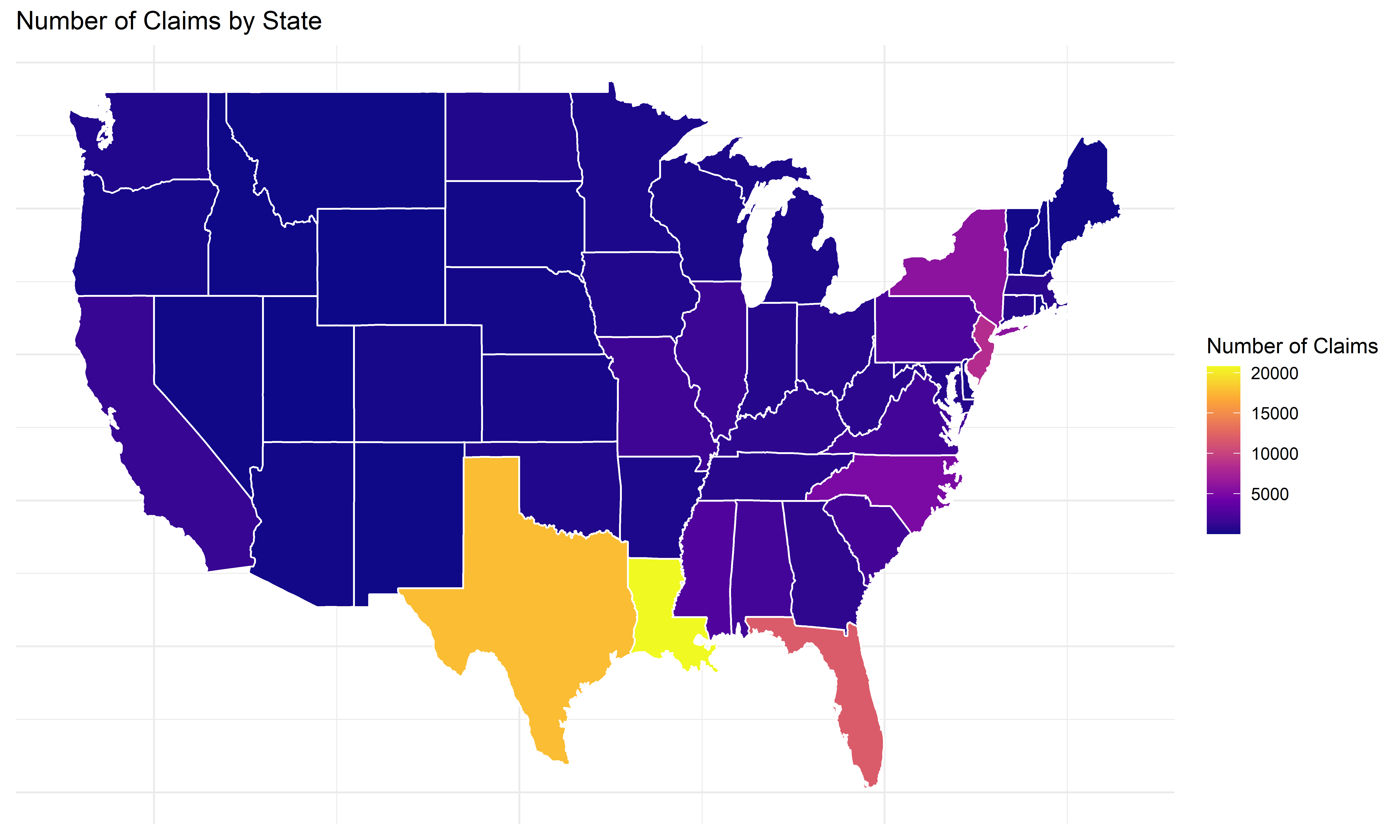
# Plot maximum claim size by state
ggplot(states_map, aes(long, lat, group = group, fill = max_claim_size)) +
  geom_polygon(color = "white") +
  scale_fill_viridis_c(option = "C") +
  labs(title = "Maximum Claim Size by State",
       fill = "Max Claim Size") +
  theme_minimal() +
  theme(axis.title = element_blank(), axis.text = element_blank(), axis.ticks = element_blank())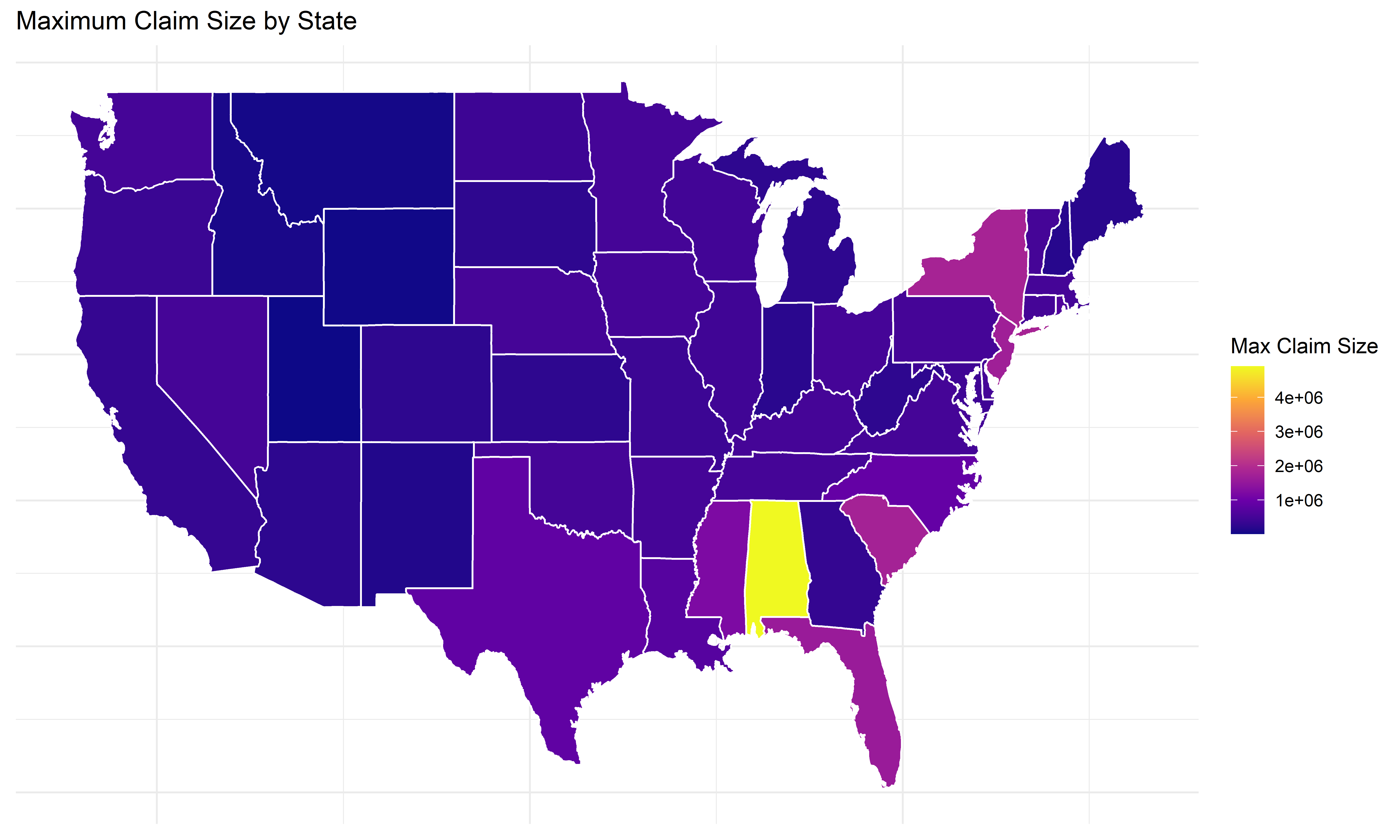
# Plot states where floods are common
ggplot(states_map, aes(long, lat, group = group, fill = common)) +
  geom_polygon(color = "white") +
  scale_fill_viridis_d() +
  labs(title = "States where flood claims are frequent",
       fill = "Number of Claims >= 1%") +
  theme_minimal() +
  theme(axis.title = element_blank(), axis.text = element_blank(), axis.ticks = element_blank())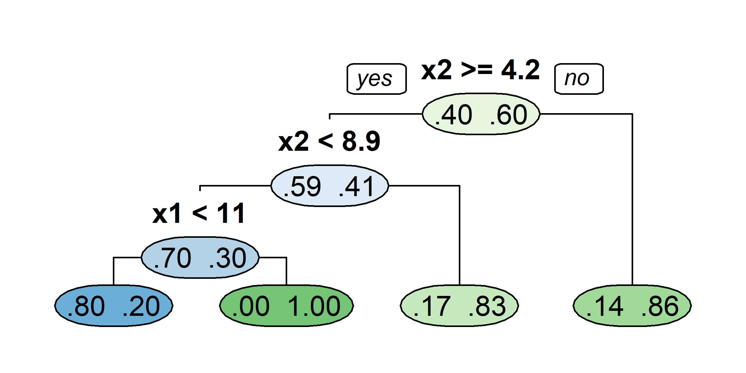


table(claims$state)
   AK    AL    AR    AZ    CA    CO    CT    DC    DE    FL    GA    GU    HI
   27  2019   410   139  1408   191   819    10   303 11833  1035     6   152
   IA    ID    IL    IN    KS    KY    LA    MA    MD    ME    MI    MN    MO
  504    43  1605   662   241  1012 20785   885   696   115   402   368  1752
   MS    MT    NC    ND    NE    NH    NJ    NM    NV    NY    OH    OK    OR
 2753    53  5023   513   189   142  8520    48    81  5899   790   490   237
   PA    PR    RI    SC    SD    TN    TX    UN    UT    VA    VI    VT    WA
 2363   569   238  2023   136   809 17759    10    11  2006    83   108   522
   WI    WV    WY
313 874 16 length(unique(claims$state))[1] 55# States with fewer than 1% claims
rare_flood_states <- names(which(table(claims[["state"]]) < nrow(claims) / 100))
claims$state <- ifelse(claims$state %in% rare_flood_states, "Other", claims$state)
table(claims$state)
   AL    CA    FL    GA    IL    KY    LA    MO    MS    NC    NJ    NY Other
 2019  1408 11833  1035  1605  1012 20785  1752  2753  5023  8520  5899 12205
   PA    SC    TX    VA
2363 2023 17759 2006 length(unique(claims$state))[1] 17tree <- rpart(amountPaidOnBuildingClaim ~ ., data=claims[1:5000,])
rpart.plot(tree)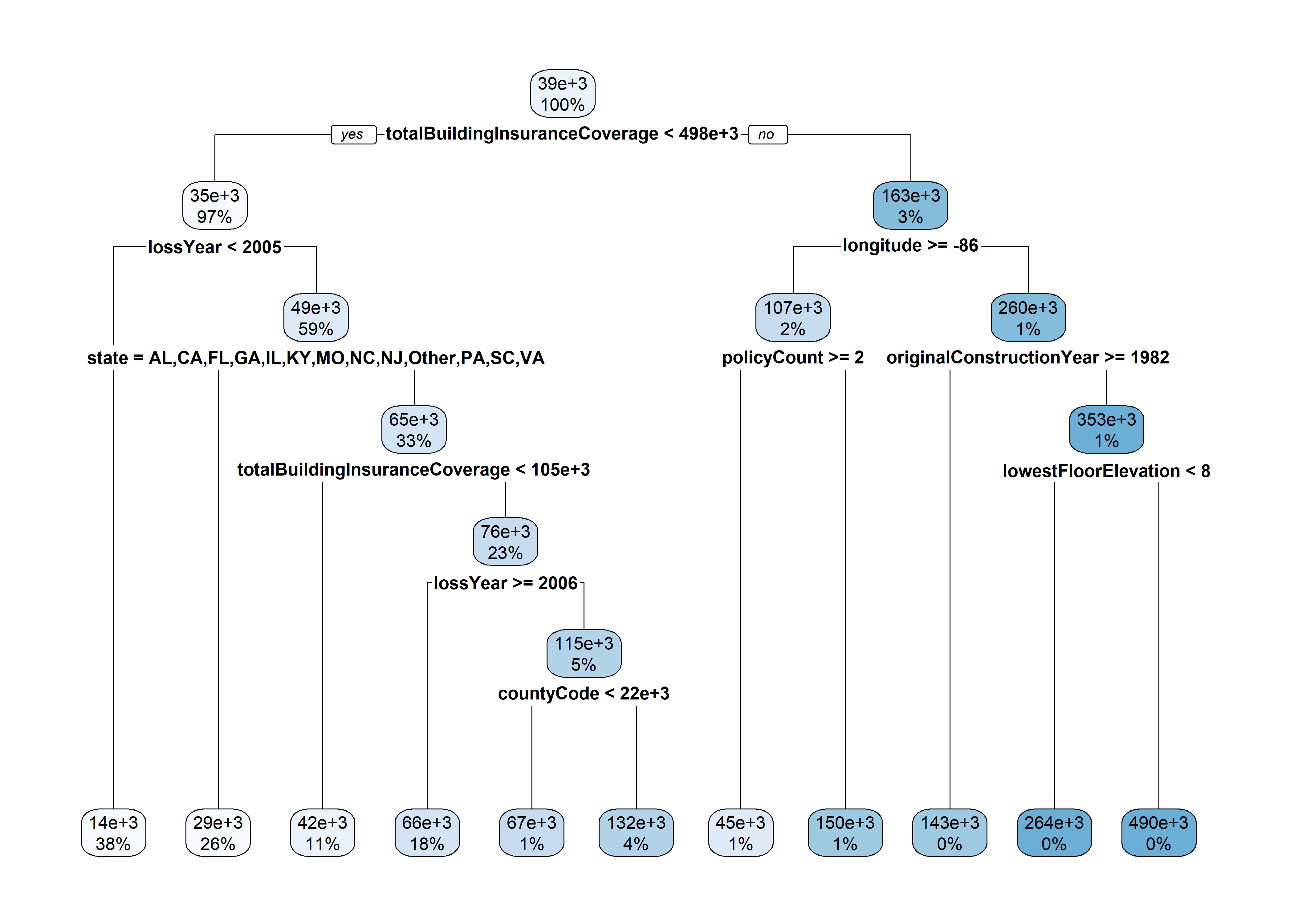
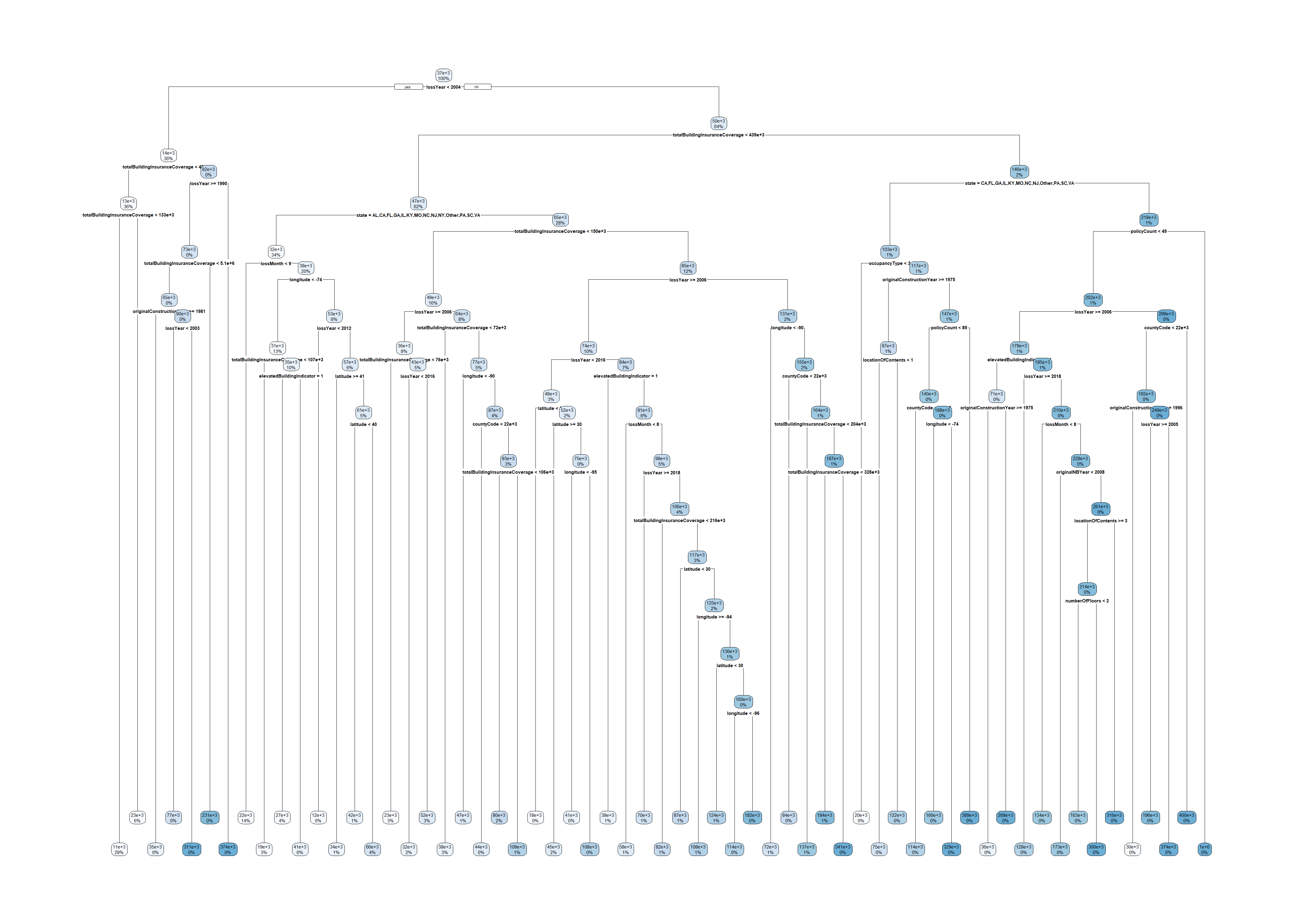
tree <- rpart(amountPaidOnBuildingClaim ~ ., data=claims[1:50000,])
rpart.plot(tree)
The smallest tree is just a root node (no splits).
The upper limit is to grow until one observation in each region.
How large should we grow the tree?

# I have already shuffled this data
train_val_index <- 1:(0.8*nrow(claims))
train_val_set <- claims[train_val_index, ]
test_set <- claims[-train_val_index, ]
train_index <- 1:(0.75*nrow(train_val_set))
train_set <- train_val_set[train_index, ]
val_set <- train_val_set[-train_index, ]
# train_set$rateMethod <- factor(train_set$rateMethod)
train_set$state <- factor(train_set$state)
# val_set$rateMethod <- factor(val_set$rateMethod, levels = levels(train_set$rateMethod))
val_set$state <- factor(val_set$state, levels = levels(train_set$state))
# test_set$rateMethod <- factor(test_set$rateMethod, levels = levels(train_set$rateMethod))
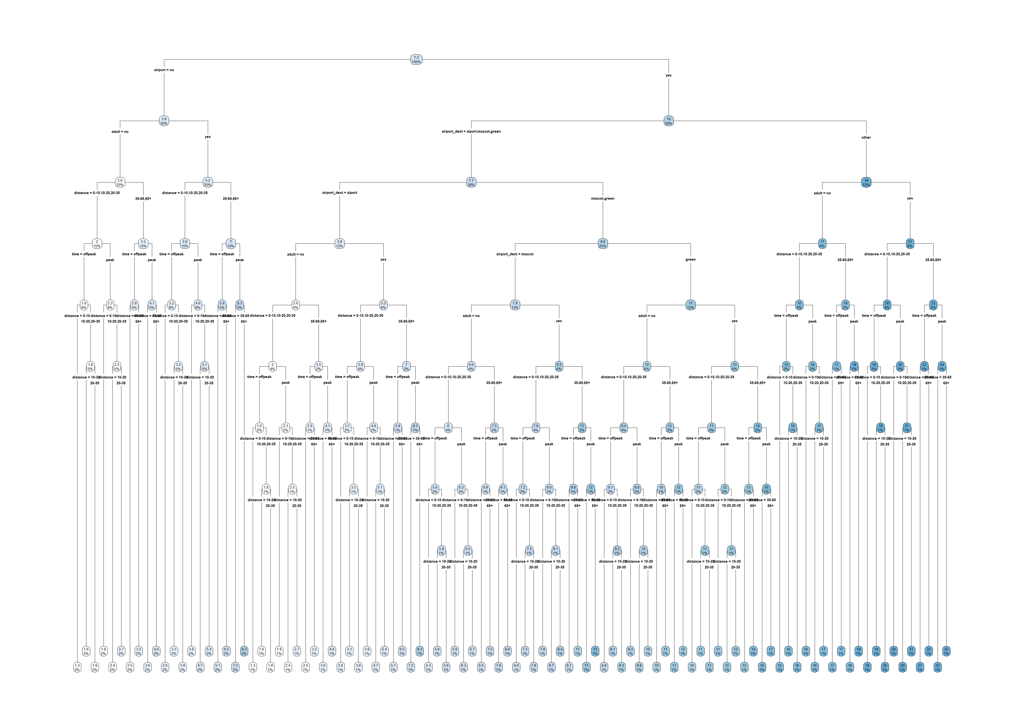
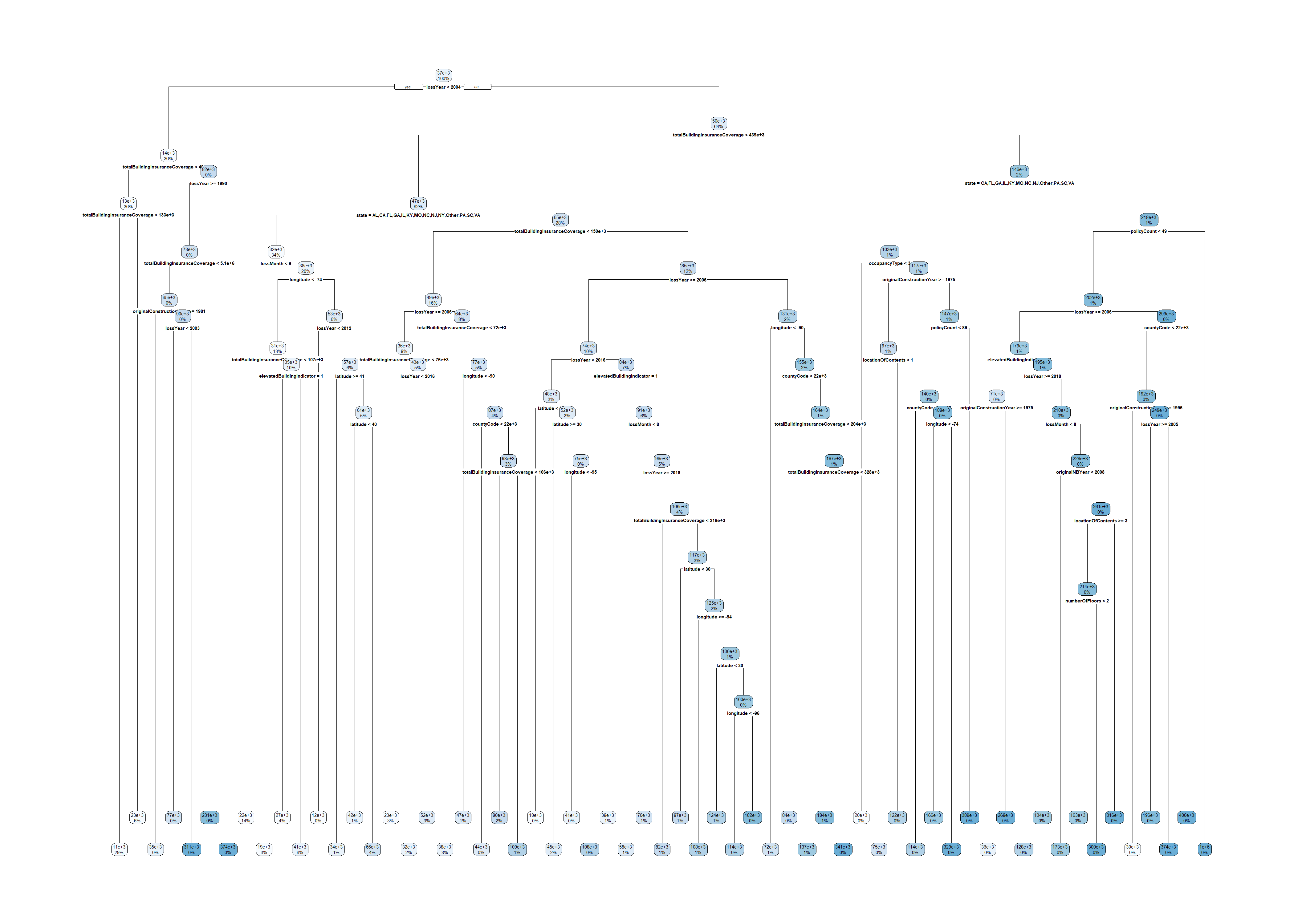
test_set$state <- factor(test_set$state, levels = levels(train_set$state))large_tree <- rpart(amountPaidOnBuildingClaim ~ ., data=train_set, control=rpart.control(cp=0.00001))
rpart.plot(large_tree)Warning: labs do not fit even at cex 0.15, there may be some overplotting
Warning: labs do not fit even at cex 0.15, there may be some overplotting
“In order to reduce the size of the tree and hence to prevent overfitting, these stopping criteria that are inherent to the recursive partitioning procedure are complemented with several rules. Three stopping rules that are commonly used can be formulated as follows:
- A node t is declared terminal when it contains less than a fixed number of observations.
- A node t is declared terminal if at least one of its children nodes t_L and t_R that results from the optimal split s_t contains less than a fixed number of observations.
- A node t is declared terminal when its depth is equal to a fixed maximal depth.”
“While the stopping rules presented above may give good results in practice, the strategy of stopping early the growing of the tree is in general unsatisfactory… That is why it is preferable to prune the tree instead of stopping the growing of the tree. Pruning a tree consists in fully developing the tree and then prune it upward until the optimal tree is found.”
Define a subtree T \subset T_0 to be any tree than can be obtained by pruning T_0 (a fully-grown tree)
Define the cost complexity criterion
\text{Total cost} = \text{Measure of Fit} + \text{Measure of Complexity}
C_\alpha(T) = \sum_{m=1}^{|T|} \sum_{i \in R_m} (y_i - \hat{y}_m)^2 + \alpha|T| where \hat{y}_m is the mean y_i in the mth leaf and \alpha controls the tradeoff between tree size and goodness of fit.
Hitters tree (only 2 predictors)Hitters example, a tree with 3 or 4 leaves (equivalently, 2 and 3 splits) is probably best.set.seed(123)
tree <- rpart(log(Salary) ~ Years + Hits, data = Hitters)
tree$cptable CP nsplit rel error xerror xstd
1 0.44457445 0 1.0000000 1.0072170 0.06567495
2 0.11454550 1 0.5554255 0.5640321 0.05904335
3 0.04446021 2 0.4408800 0.4620370 0.05746429
4 0.01831268 3 0.3964198 0.4290060 0.05941502
5 0.01690198 4 0.3781072 0.4329760 0.06391180
6 0.01107214 5 0.3612052 0.4329270 0.06603000
7 0.01000000 6 0.3501330 0.4445006 0.06621925plotcp(tree)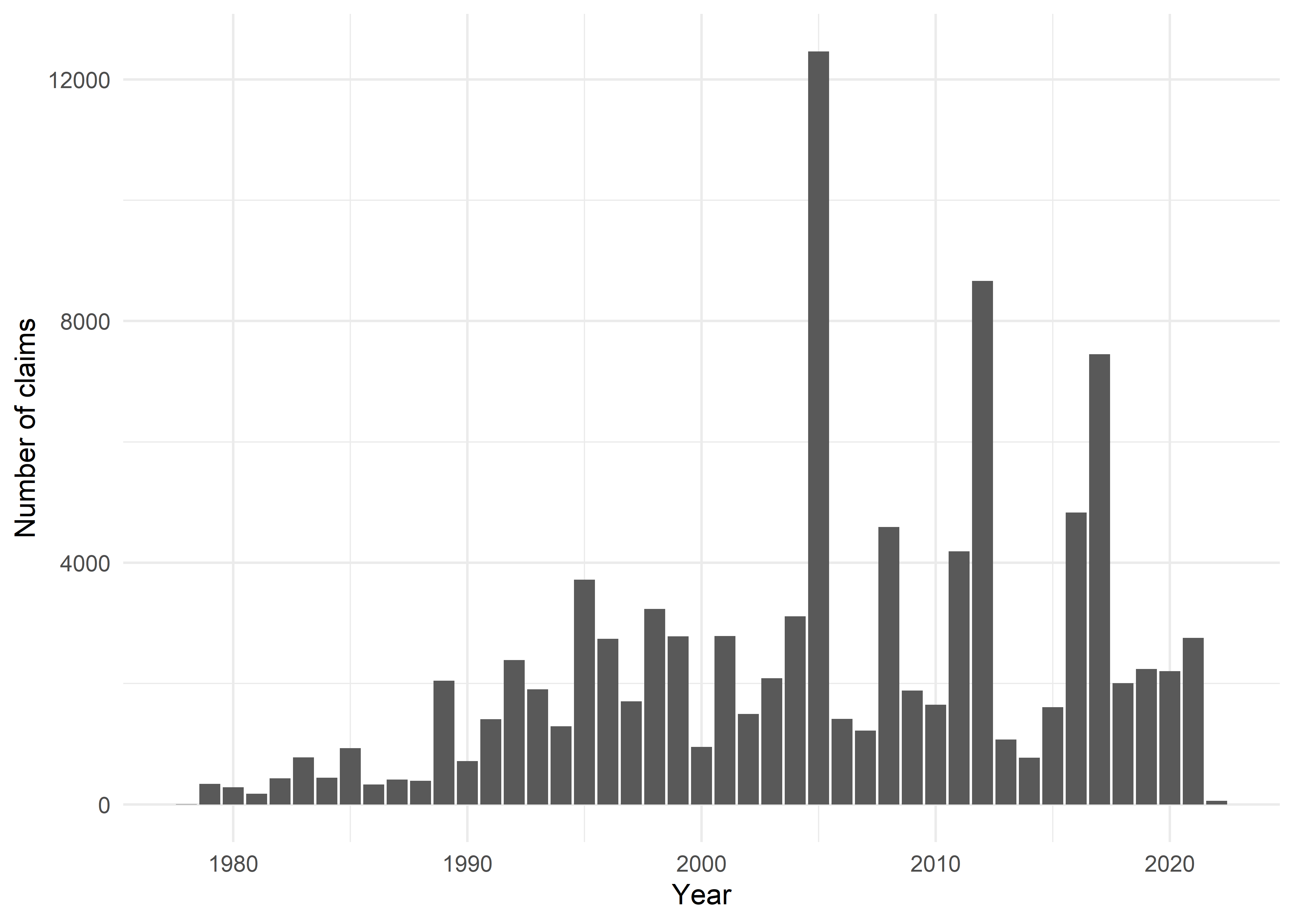
Hitters tree: all predictors

# Perform cross-validation to prune the tree
set.seed(123)
cv_tree <- train(
  amountPaidOnBuildingClaim ~ .,
  data=train_set,
  method="rpart",
  trControl=trainControl(method="cv", number=5),
  tuneGrid=data.frame(cp=seq(0, 0.01, 0.001))
)
# Get the optimal cp value
optimal_cp <- cv_tree$bestTune$cp
plot(cv_tree)
pruned_tree <- prune(large_tree, cp=optimal_cp)
rpart.plot(pruned_tree)
Warning: labs do not fit even at cex 0.15, there may be some overplotting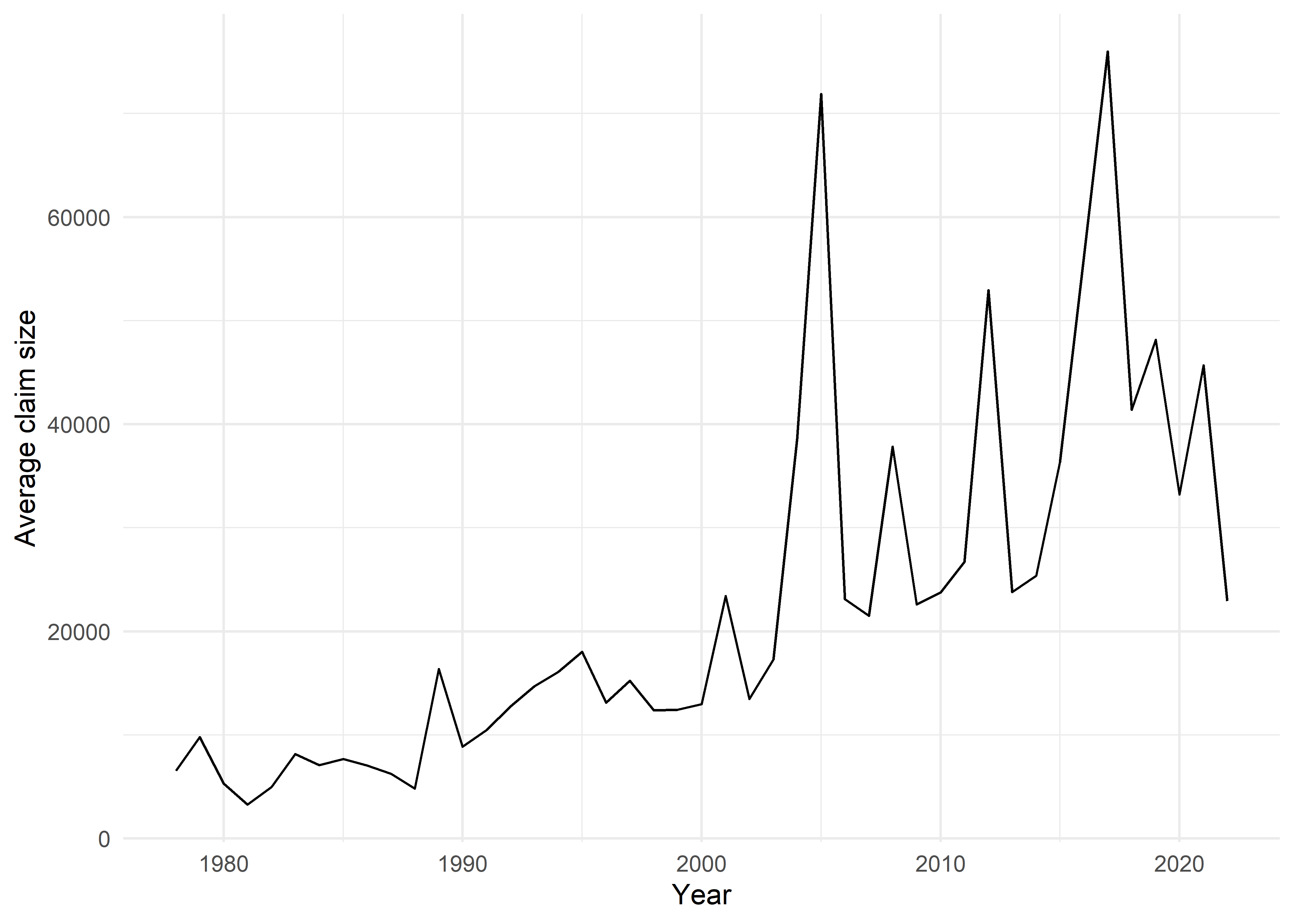
linear <- lm(amountPaidOnBuildingClaim ~ ., data=train_set)
summary(linear)
Call:
lm(formula = amountPaidOnBuildingClaim ~ ., data = train_set)

Residuals:
    Min      1Q  Median      3Q     Max
-785390  -27448  -10894   11246 4787232

Coefficients:
                                 Estimate Std. Error t value Pr(>|t|)
(Intercept)                    -2.793e+06  6.662e+04 -41.928  < 2e-16 ***
agricultureStructureIndicator   1.662e+04  1.669e+04   0.996 0.319163
policyCount                     1.463e+03  1.179e+02  12.407  < 2e-16 ***
countyCode                      6.958e-02  3.986e-02   1.746 0.080900 .
elevatedBuildingIndicator      -1.387e+04  6.202e+02 -22.358  < 2e-16 ***
latitude                        3.955e+02  1.031e+02   3.835 0.000125 ***
locationOfContents              4.392e+02  1.412e+02   3.111 0.001864 **
longitude                      -1.455e+02  3.953e+01  -3.681 0.000232 ***
lowestFloorElevation           -4.797e-02  5.281e-01  -0.091 0.927623
occupancyType                   3.937e+03  1.681e+02  23.413  < 2e-16 ***
postFIRMConstructionIndicator   3.291e+03  7.311e+02   4.501 6.78e-06 ***
stateCA                        -8.250e+03  2.975e+03  -2.773 0.005548 **
stateFL                        -1.210e+04  1.873e+03  -6.459 1.07e-10 ***
stateGA                        -1.194e+04  2.955e+03  -4.040 5.36e-05 ***
stateIL                        -2.142e+04  2.859e+03  -7.494 6.80e-14 ***
stateKY                        -1.385e+04  3.145e+03  -4.405 1.06e-05 ***
stateLA                         1.495e+04  1.944e+03   7.688 1.52e-14 ***
stateMO                        -1.212e+04  2.888e+03  -4.198 2.70e-05 ***
stateMS                         2.054e+04  2.442e+03   8.410  < 2e-16 ***
stateNC                        -1.536e+04  2.588e+03  -5.935 2.95e-09 ***
stateNJ                        -9.051e+03  2.700e+03  -3.353 0.000801 ***
stateNY                        -4.034e+03  2.869e+03  -1.406 0.159733
stateOther                     -1.757e+04  2.507e+03  -7.006 2.48e-12 ***
statePA                        -1.705e+04  3.180e+03  -5.360 8.37e-08 ***
stateSC                        -1.064e+04  2.999e+03  -3.549 0.000387 ***
stateTX                         4.916e+03  2.589e+03   1.898 0.057665 .
stateVA                        -2.123e+04  3.337e+03  -6.363 1.99e-10 ***
totalBuildingInsuranceCoverage -1.912e-03  6.089e-04  -3.140 0.001693 **
numberOfFloors                 -5.613e+01  3.050e+02  -0.184 0.854001
lossYear                        1.400e+03  4.691e+01  29.845  < 2e-16 ***
lossMonth                       2.253e+03  1.018e+02  22.130  < 2e-16 ***
originalConstructionYear        5.103e+00  2.298e+01   0.222 0.824242
originalConstructionMonth      -8.065e+01  7.097e+01  -1.136 0.255851
originalNBYear                 -1.772e+01  4.758e+01  -0.372 0.709551
originalNBMonth                 1.601e+01  7.470e+01   0.214 0.830288
---
Signif. codes:  0 '***' 0.001 '**' 0.01 '*' 0.05 '.' 0.1 ' ' 1

Residual standard error: 57740 on 59965 degrees of freedom
Multiple R-squared:  0.1328,    Adjusted R-squared:  0.1323
F-statistic: 270 on 34 and 59965 DF, p-value: < 2.2e-16| Method | Test RMSE |
|---|---|
| Linear Model | 5.4792^{4} |
| Large Tree | 4.8683^{4} |
| Pruned Tree | 4.7372^{4} |
Advantages
Disadvantages
Is there a way to improve the predictive performance of trees?
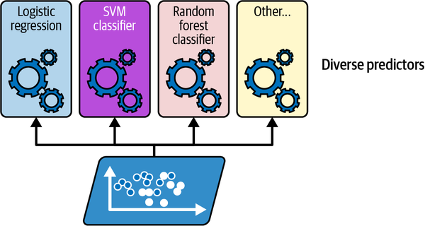
Original dataset
# Sort by first column to make
# it easier to see the resampling
# (so not necessary in general).
df %>% arrange(x1)
A bootstrap resample
set.seed(1)
df %>%
  sample_n(size=nrow(df), replace=TRUE) %>%
  arrange(x1)
There are 54% of the rows in the original dataset in the bootstrap resample.
Original dataset
# Sort by first column to make
# it easier to see the resampling
# (so not necessary in general).
df %>% arrange(x1)
A bootstrap resample
set.seed(4)
df %>%
  sample_n(size=nrow(df), replace=TRUE) %>%
  arrange(x1)
There are 68% of the rows in the original dataset in the bootstrap resample.
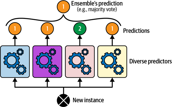
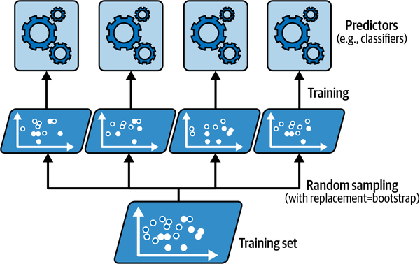
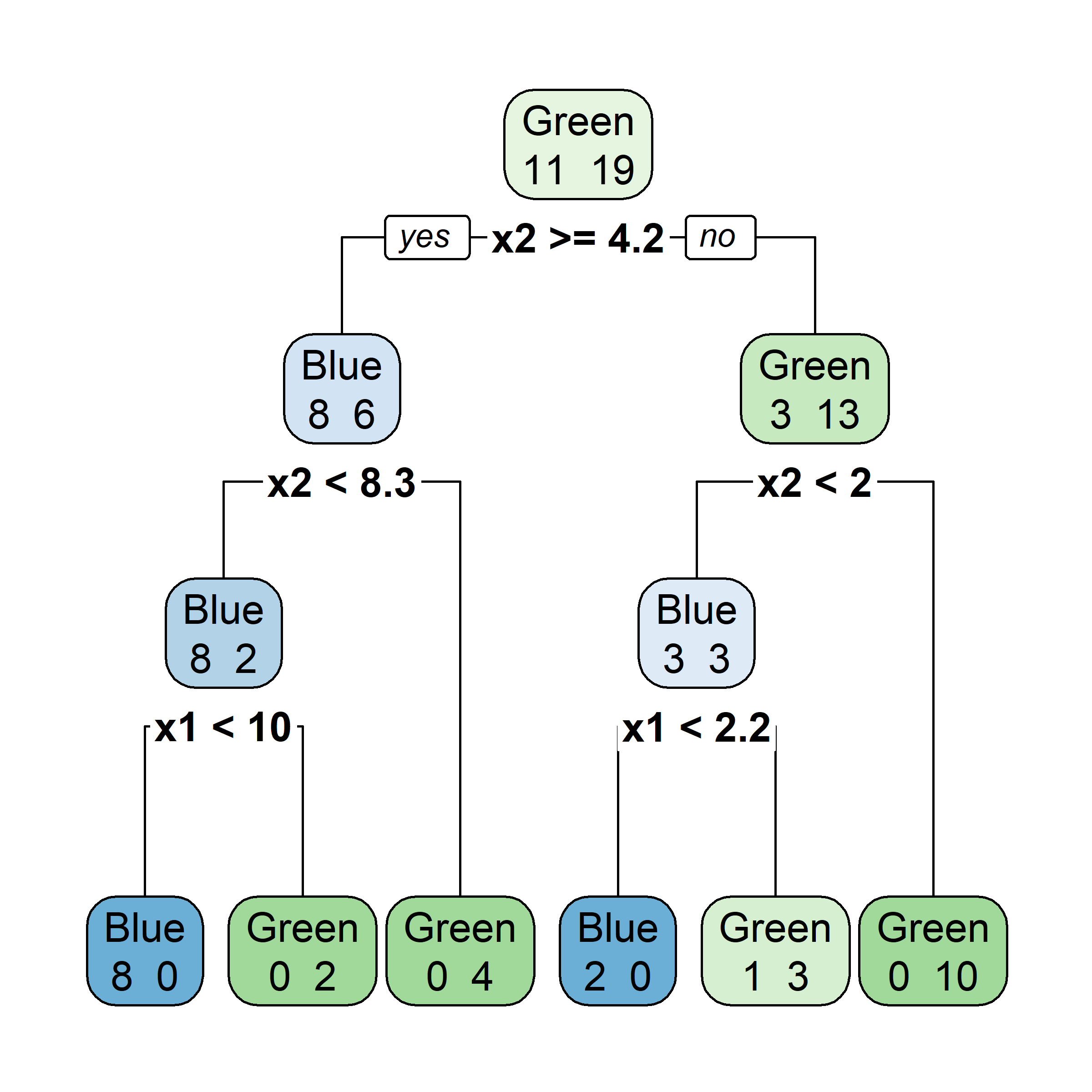
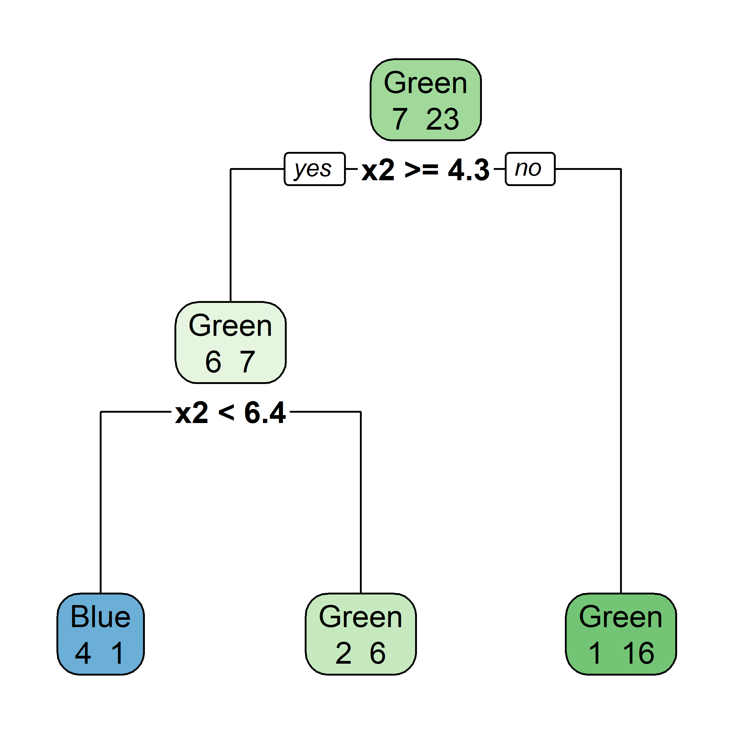
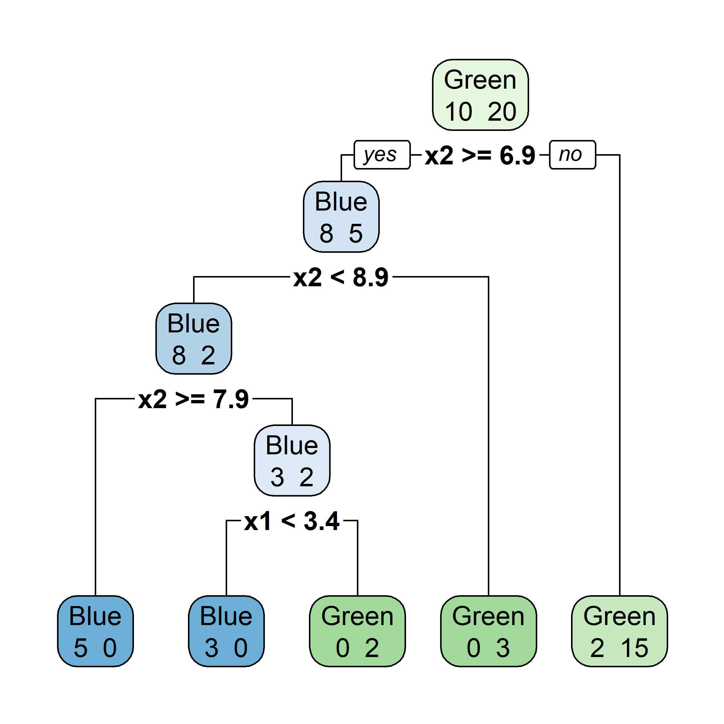
Bagging procedure for trees:
Let’s say element i,j of the matrix is 1 if the ith observation is in the jth bootstrap sample (we say it is “in the bag”) and 0 otherwise.
Now consider the inverse, element i,j of the matrix is 1 if the ith observation is not in the jth bootstrap sample, it is “out of the bag”.
This provides a simple way to estimate the test error of the bagged model: “out-of-bag error” (cheaper than cross-validation).
There is a very straightforward way to estimate the test error of a bagged model

randomForestrf_model <- randomForest(amountPaidOnBuildingClaim ~ ., data = train_set,
ntree=50, importance = TRUE)# Calculate validation set RMSE
val_pred <- predict(rf_model, newdata=val_set)
val_rmse_rf <- sqrt(mean((val_pred - val_set$amountPaidOnBuildingClaim)^2))| Method | RMSE |
|---|---|
| Linear Model | 5.4792^{4} |
| Large Tree | 4.8683^{4} |
| Pruned Tree | 4.7372^{4} |
| Random Forest | 4.2829^{4} |
importance(rf_model) %IncMSE IncNodePurity
agricultureStructureIndicator -0.4092969 7.736630e+10
policyCount -0.6649637 1.312233e+13
countyCode 7.0676498 1.261540e+13
elevatedBuildingIndicator 1.9163476 4.066224e+12
latitude 12.7351805 1.257793e+13
locationOfContents 1.2897842 5.107086e+12
longitude 15.2725053 1.588849e+13
lowestFloorElevation 0.5264056 8.837304e+12
occupancyType -0.8955214 5.325440e+12
postFIRMConstructionIndicator 12.1436127 1.855385e+12
state 10.2933401 1.275269e+13
totalBuildingInsuranceCoverage 8.0324394 4.040641e+13
numberOfFloors 11.7156439 3.504747e+12
lossYear 8.2085826 2.277261e+13
lossMonth 17.4917355 1.009505e+13
originalConstructionYear 9.4747850 1.235049e+13
originalConstructionMonth 2.8065239 6.062158e+12
originalNBYear 6.7318799 1.468756e+13
originalNBMonth 1.5024842 1.277571e+13varImpPlot(rf_model)
Note: the final model can be expressed as: \hat{f}(x) = \sum_{b=1}^{B}\lambda \hat{f}^b(x).
gbm# Fit a gradient boosting model
gbm_model <- gbm(amountPaidOnBuildingClaim ~ ., data = train_set,
distribution = "gaussian", n.trees = 5000,
interaction.depth = 2, shrinkage = 0.01, cv.folds = 5)
best_iter <- gbm.perf(gbm_model, method = "cv")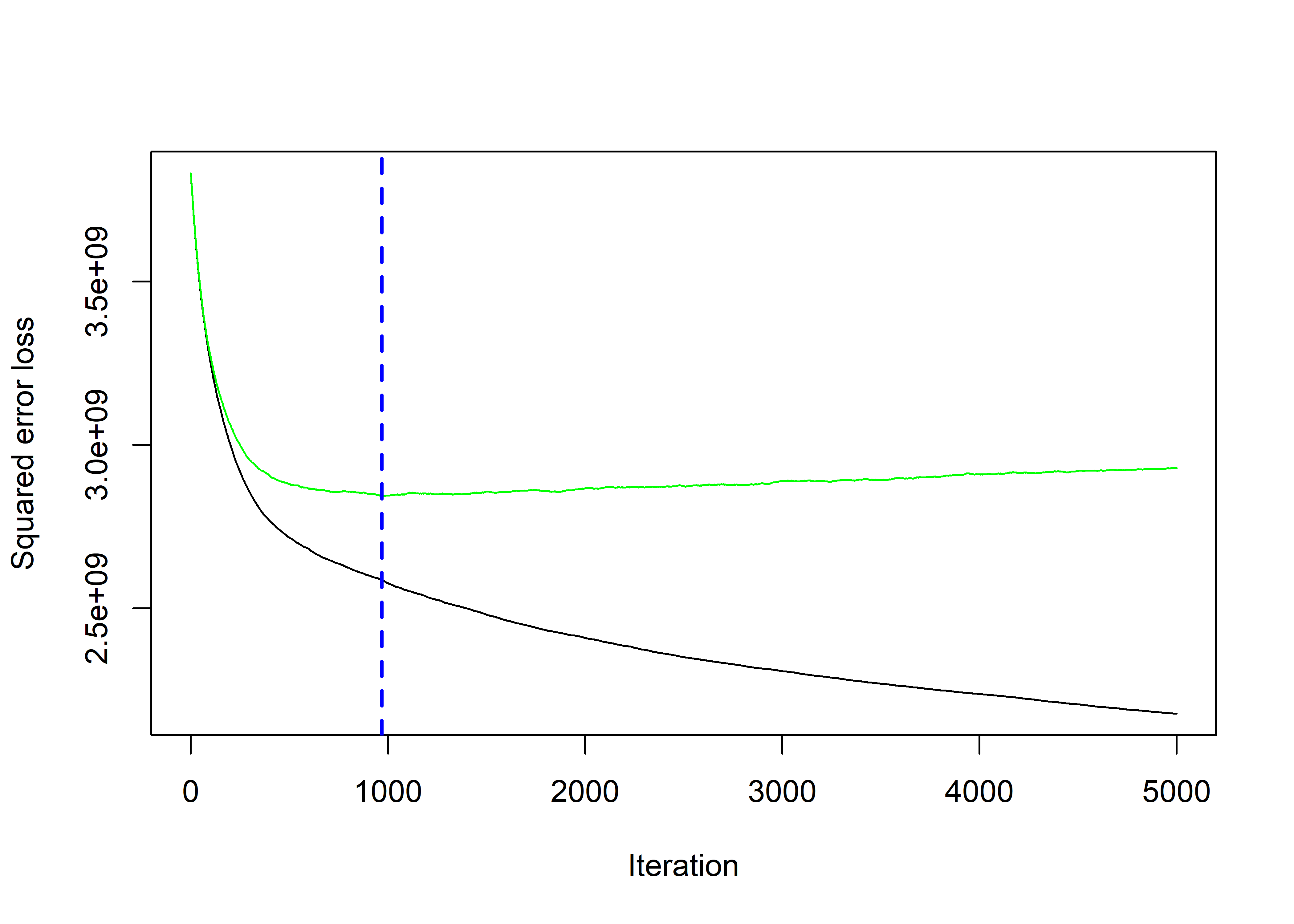
predictions <- predict(gbm_model, newdata = val_set, n.trees = best_iter)| Method | RMSE |
|---|---|
| Linear Model | 5.4792^{4} |
| Gradient Boosting | 4.982^{4} |
| Large Tree | 4.8683^{4} |
| Pruned Tree | 4.7372^{4} |
| Random Forest | 4.2829^{4} |
Finally, evaluating the winning model on the test set:
if (val_rmse_gbm < val_rmse_rf) {
  predictions <- predict(gbm_model, newdata = test_set, n.trees = best_iter)
  test_rmse <- sqrt(mean((predictions - test_set$amountPaidOnBuildingClaim)^2))
} else {
  predictions <- predict(rf_model, newdata = test_set)
  test_rmse <- sqrt(mean((predictions - test_set$amountPaidOnBuildingClaim)^2))
}
round(test_rmse)
[1] 44468Test set root mean-squared error for the winning model is 4.4468495^{4}.
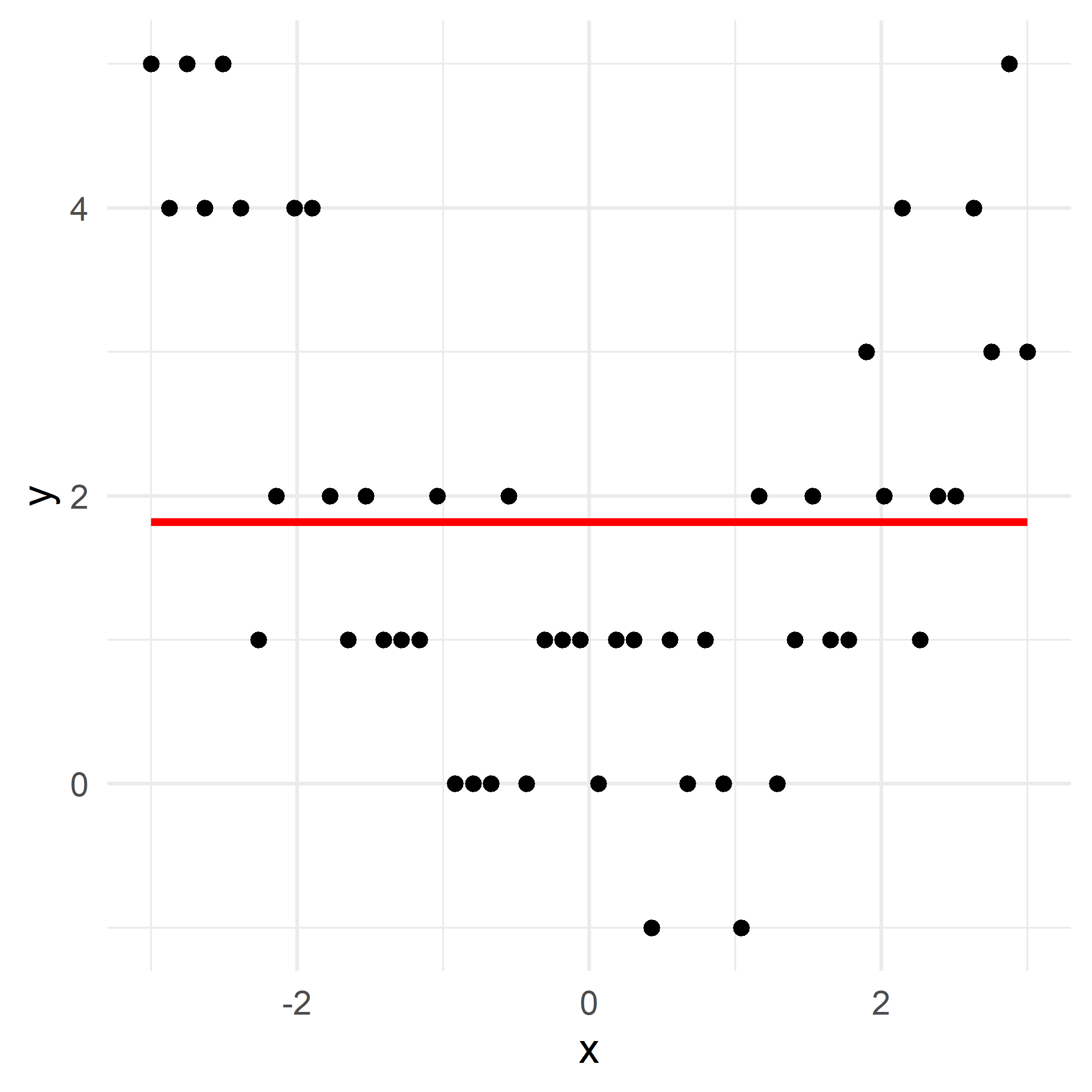
x_obs = np.linspace(-3, 3, 50)
y_obs = [5, 4, 5, 4, 5, 4, 1, 2, 4, 4, 2, 1, 2, 1, 1, 1, 2, 0, 0, 0, 2, 0, 1, 1, 1, 0, 1, 1, -1, 1, 0, 1, 0, -1, 2, 0, 1, 2, 1, 1, 3, 2, 4, 1, 2, 2, 4, 3, 5, 3]
df = pd.DataFrame({'x': x_obs, 'y': y_obs})
# Parameters
d = 1 # number of splits
lambda_ = 0.5 # learning rate
# Higher resolution grid
x_obs = x_obs.reshape(-1, 1)
x_grid = np.linspace(-3, 3, 1000)
# Initial model
f_hat = np.zeros_like(df['y'], dtype=float)
residuals = df['y'].astype(float).copy()
# Store predictions for the grid
f_hat_grid = np.zeros_like(x_grid, dtype=float)
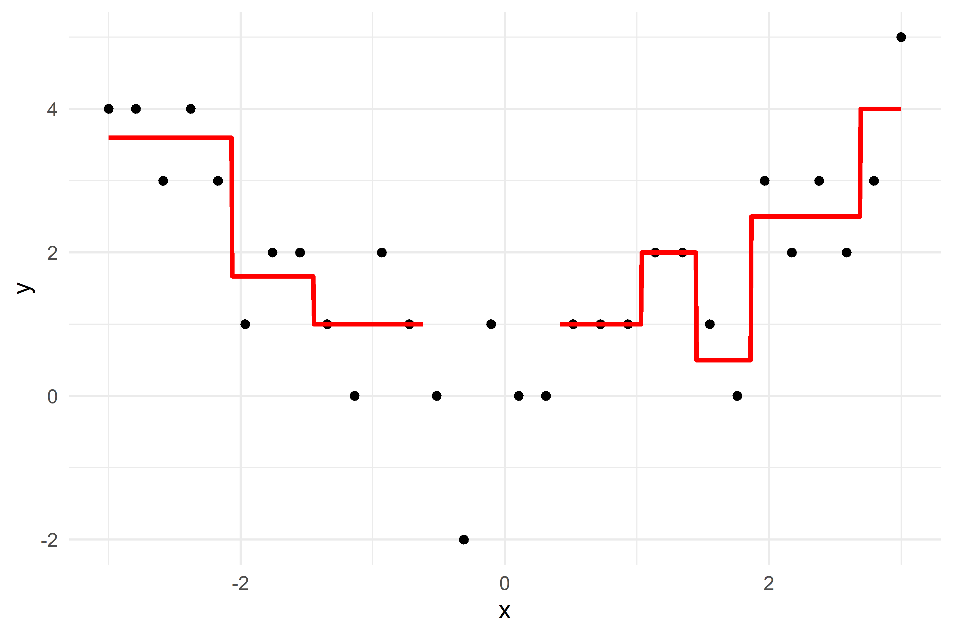
def plot_boosting_iteration(df, x_grid, f_hat, residuals, f_hat_grid, d, lambda_):
fig, axes = plt.subplots(1, 3, figsize=(10, 4))
# Plot residuals
axes[0].scatter(df['x'], residuals, color='blue', label='Residuals')
axes[0].plot(x_grid, f_b_grid, color='green', label='New Tree')
axes[0].set_ylim(-1.25, 5.25)
axes[0].set_title(f"Residuals")
# Plot updated model prediction
axes[1].plot(x_grid, f_hat_grid, color='purple')
axes[1].scatter(df['x'], df['y'], color='red', alpha=0.5)
axes[1].set_ylim(-1.25, 5.25)
axes[1].set_title(f"Updated Prediction")
# Plot new residuals
axes[2].scatter(df['x'], df['y'] - f_hat, color='blue', label='Residuals')
axes[2].set_ylim(-1.25, 5.25)
axes[2].set_title(f"New Residuals")
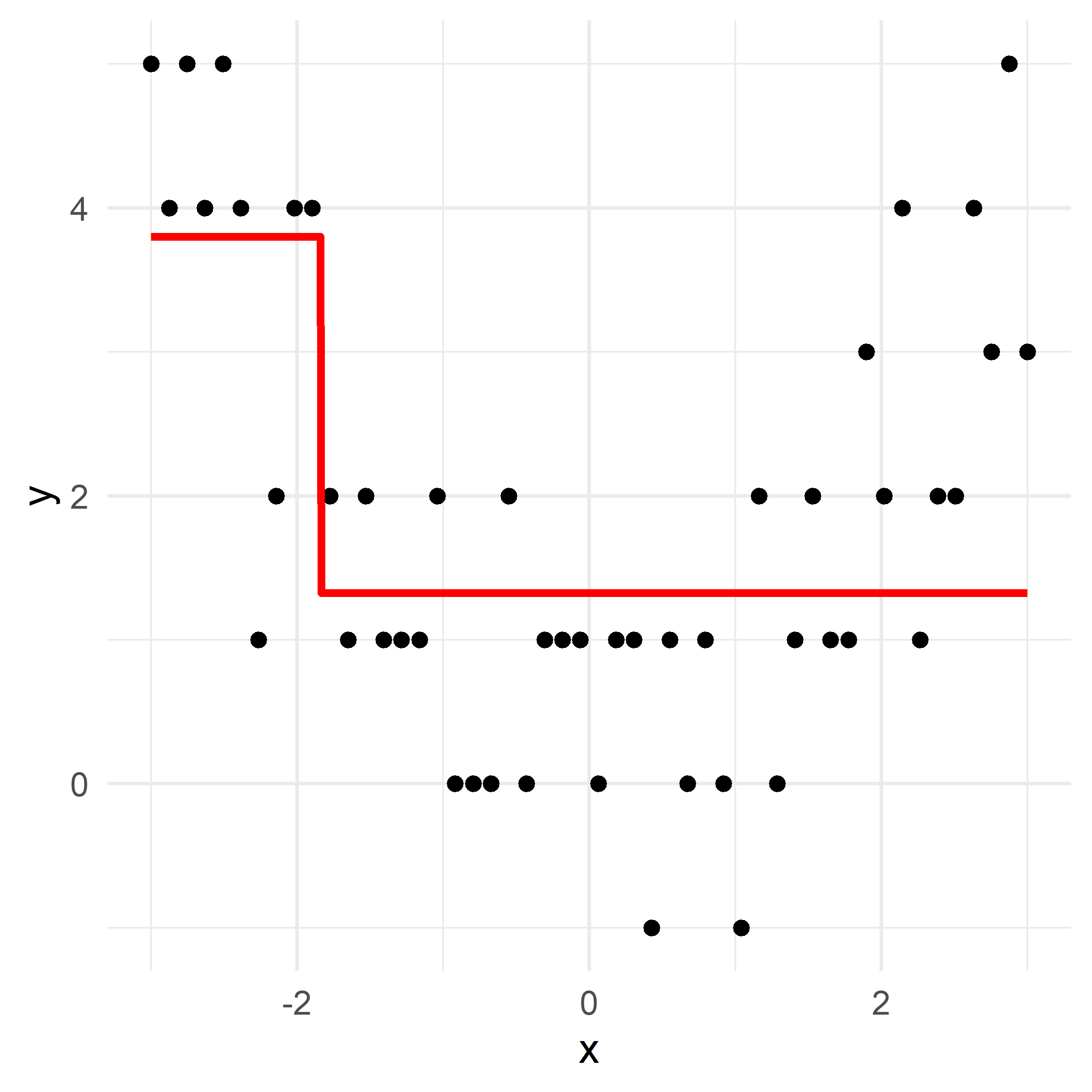
plt.tight_layout()# Fit a tree to residuals
tree = DecisionTreeRegressor(max_depth=d)
tree.fit(x_obs, residuals);
f_b = tree.predict(x_obs)
f_b_grid = tree.predict(x_grid.reshape(-1, 1))
# Update model
f_hat += lambda_ * f_b
f_hat_grid += lambda_ * f_b_grid
plot_boosting_iteration(df, x_grid, f_hat, residuals, f_hat_grid, d, lambda_)
# Update residuals
residuals -= lambda_ * f_b
Here, \lambda=\frac12 is the learning rate.
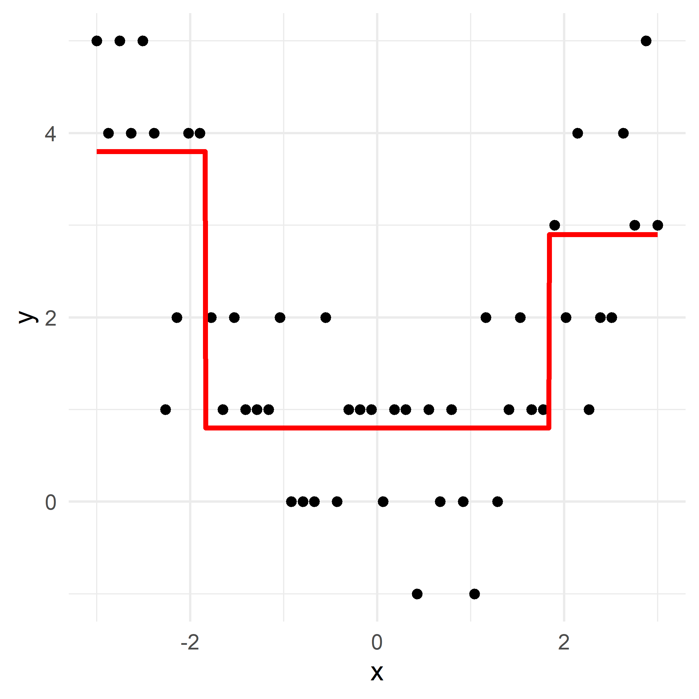
# Fit a tree to residuals
tree = DecisionTreeRegressor(max_depth=d)
tree.fit(x_obs, residuals);
f_b = tree.predict(x_obs)
f_b_grid = tree.predict(x_grid.reshape(-1, 1))

# Update model
f_hat += lambda_ * f_b
f_hat_grid += lambda_ * f_b_grid
plot_boosting_iteration(df, x_grid, f_hat, residuals, f_hat_grid, d, lambda_)

# Update residuals
residuals -= lambda_ * f_b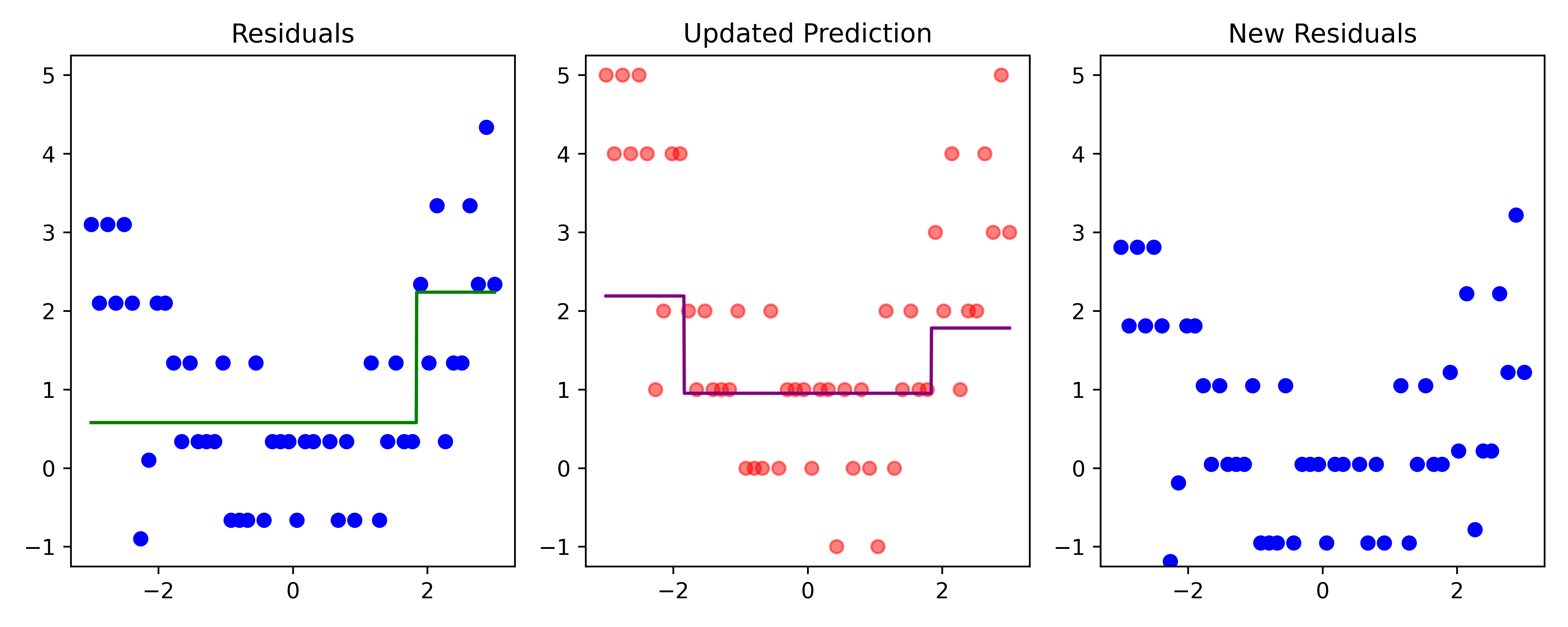
Here, \lambda=\frac12 is the learning rate.
# Fit a tree to residuals
tree = DecisionTreeRegressor(max_depth=d)
tree.fit(x_obs, residuals);
f_b = tree.predict(x_obs)
f_b_grid = tree.predict(x_grid.reshape(-1, 1))

# Update model
f_hat += lambda_ * f_b
f_hat_grid += lambda_ * f_b_grid
plot_boosting_iteration(df, x_grid, f_hat, residuals, f_hat_grid, d, lambda_)

# Update residuals
residuals -= lambda_ * f_b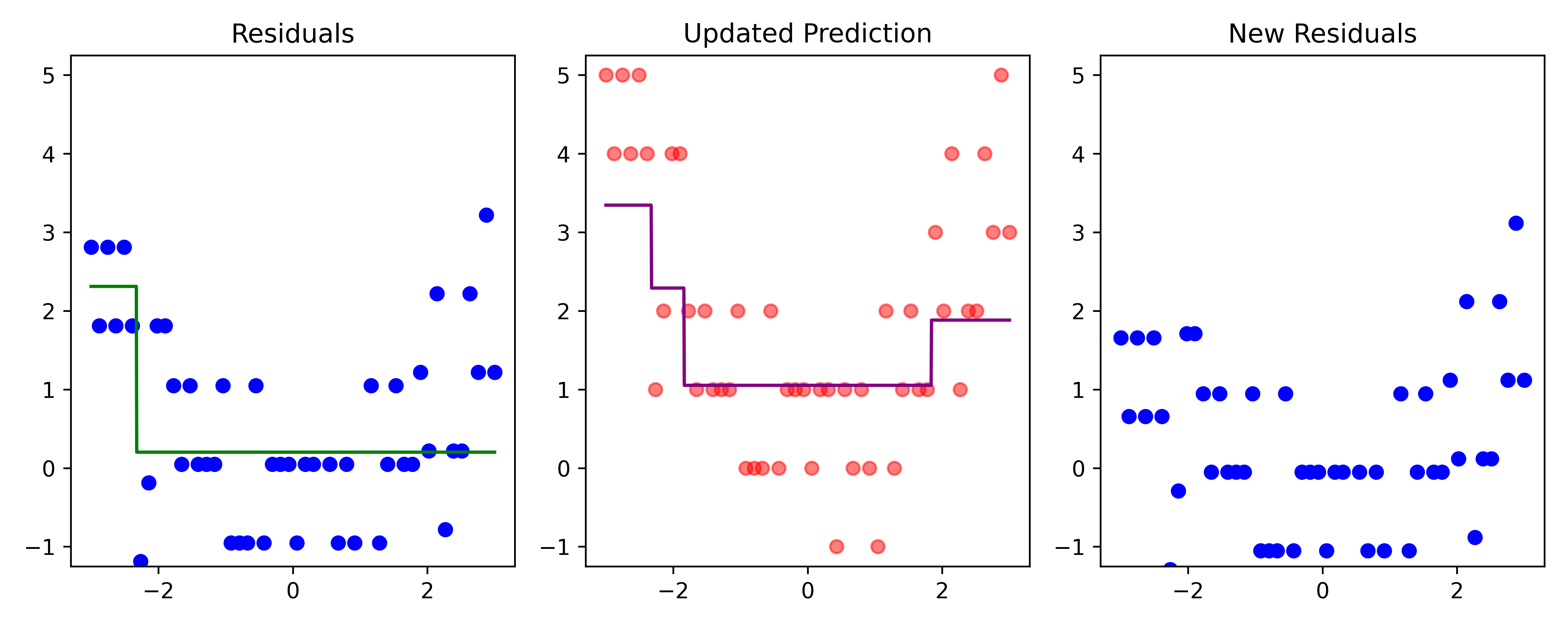
Here, \lambda=\frac12 is the learning rate.
# Fit a tree to residuals
tree = DecisionTreeRegressor(max_depth=d)
tree.fit(x_obs, residuals);
f_b = tree.predict(x_obs)
f_b_grid = tree.predict(x_grid.reshape(-1, 1))

# Update model
f_hat += lambda_ * f_b
f_hat_grid += lambda_ * f_b_grid
plot_boosting_iteration(df, x_grid, f_hat, residuals, f_hat_grid, d, lambda_)

# Update residuals
residuals -= lambda_ * f_b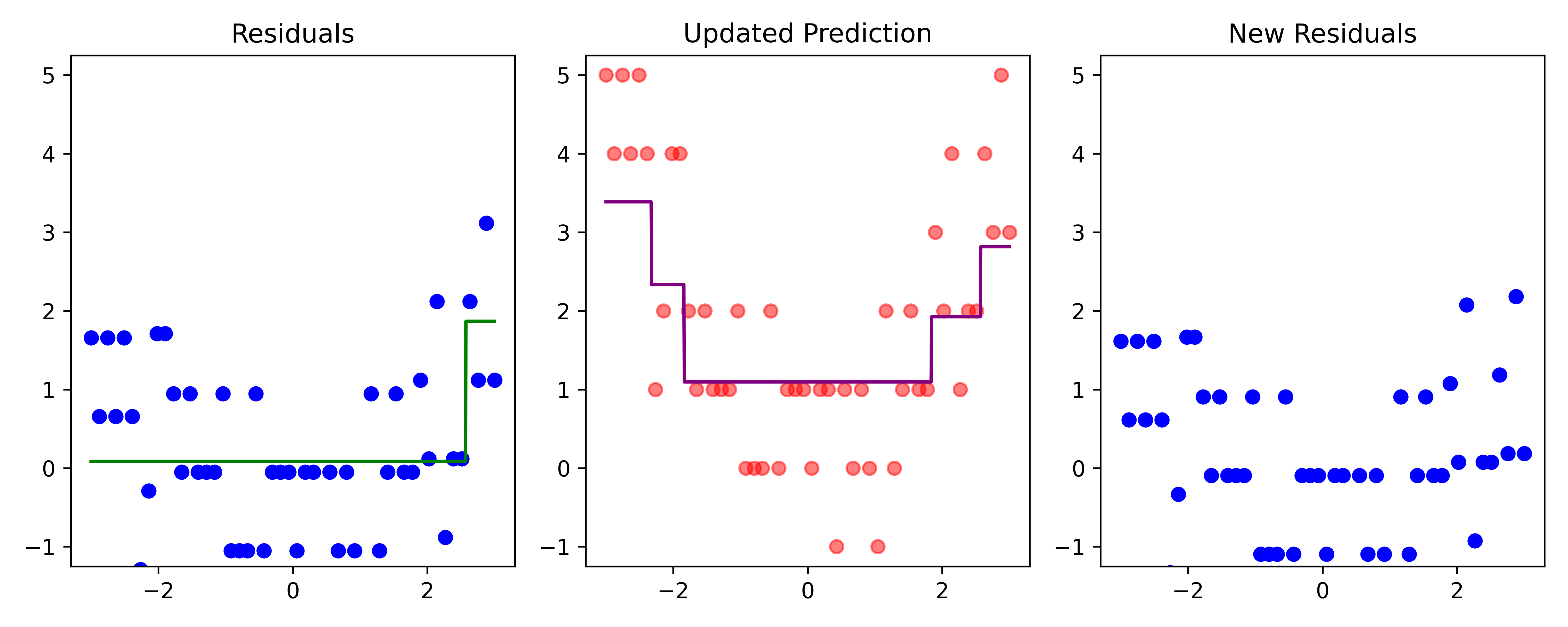
Here, \lambda=\frac12 is the learning rate.
# Fit a tree to residuals
tree = DecisionTreeRegressor(max_depth=d)
tree.fit(x_obs, residuals);
f_b = tree.predict(x_obs)
f_b_grid = tree.predict(x_grid.reshape(-1, 1))

# Update model
f_hat += lambda_ * f_b
f_hat_grid += lambda_ * f_b_grid
plot_boosting_iteration(df, x_grid, f_hat, residuals, f_hat_grid, d, lambda_)

# Update residuals
residuals -= lambda_ * f_b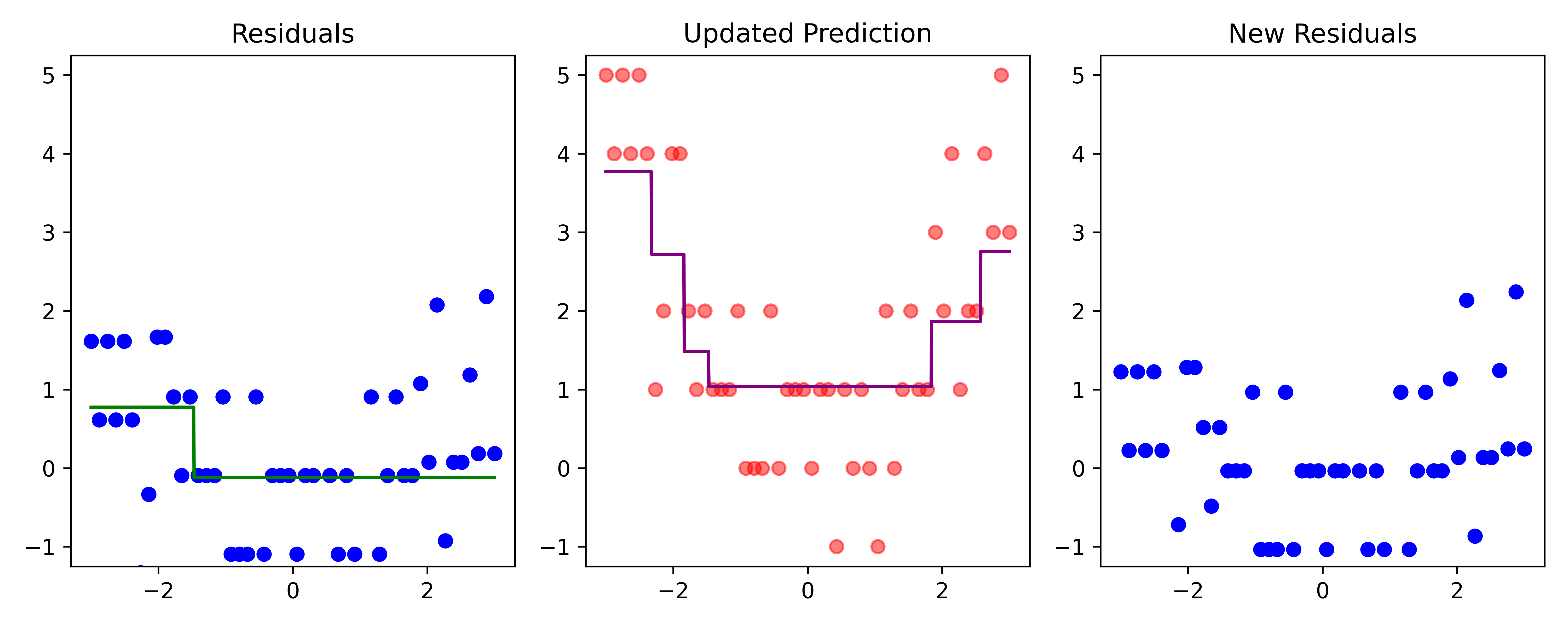
Here, \lambda=\frac12 is the learning rate.