set.seed(1)
x1 <- runif(100)
x2 <- 0.5 * x1 + rnorm(100) / 10
y <- 2 + 2 * x1 + 0.3 * x2 + rnorm(100)Lab 3: Multiple Linear Regression
Multiple Predictors, Model Selection & Issues with Linear Regression
Questions
Conceptual Questions
Solution Refer to Table 3.4 in the ISL textbook (James et al., 2021). Describe the null hypotheses to which the p-values in the Table correspond. Explain what conclusions you can draw based on these p-values. Your explanation should be phrased in terms of
sales,TV,radio, andnewspaper, rather than in terms of the coefficients of the linear model.\star Solution I collect a set of data (n = 100 observations) containing a single predictor and a quantitative response. I then fit a linear regression model to the data, as well as a separate cubic regression, i.e. Y =\beta_0 + \beta_1 X + \beta_2 X^2 + \beta_3 X^3 + \epsilon.
Suppose that the true relationship between X and Y is linear, i.e. Y = \beta_0 + \beta_1 X + \epsilon. Consider the training residual sum of squares (RSS) for the linear regression, and also the training RSS for the cubic regression. Would we expect one to be lower than the other, would we expect them to be the same, or is there not enough information to tell? Justify your answer.
Answer (a) using test rather than training RSS.
Suppose that the true relationship between X and Y is not linear, but we don’t know how far it is from linear. Consider the training RSS for the linear regression, and also the training RSS for the cubic regression. Would we expect one to be lower than the other, would we expect them to be the same, or is there not enough information to tell? Justify your answer.
Answer (c) using test rather than training RSS.
-
Write out the design matrix \boldsymbol{X} in the special case of the simple linear regression model (i.e., one predictor).
Write out the matrix \boldsymbol{X}^\top\boldsymbol{X} for the simple linear regression model.
Write out the vector \boldsymbol{X}^\top\boldsymbol{y} for the simple linear regression model.
Write out the matrix (\boldsymbol{X}^\top\boldsymbol{X})^{-1} for the simple linear regression model.
Calculate \widehat{\boldsymbol{\beta}}=(\boldsymbol{X}^\top\boldsymbol{X})^{-1}\boldsymbol{X}^\top\boldsymbol{y} using your results above.
Where \boldsymbol{y} is the vector of the response variable and \boldsymbol{\widehat{\beta}} is the vector of coefficients.
\star Solution The following model was fitted to a sample of supermarkets in order to explain their profit levels: y=\beta_{0} + \beta_{1} x_{1} + \beta_{2} x_{2} + \beta_{3} x_{3} + \varepsilon where
y= profits, in thousands of dollars
x_{1}= food sales, in tens of thousands of dollars
x_{2}= nonfood sales, in tens of thousands of dollars, and
x_{3}= store size, in thousands of square feet.
The estimated regression coefficients are given below: \widehat{\beta}_{1} = 0.027 \text{ and } \widehat{\beta}_{2} = -0.097 \text{ and } \widehat{\beta}_{3} = 0.525.
Which of the following is TRUE?
A dollar increase in food sales increases profits by 2.7 cents.
A 2.7 cent increase in food sales increases profits by a dollar.
A 9.7 cent increase in nonfood sales decreases profits by a dollar.
A dollar decrease in nonfood sales increases profits by 9.7 cents.
An increase in store size by one square foot increases profits by 52.5 cents.
\star Solution In a regression model of three explanatory variables, twenty-five observations were used to calculate the least squares estimates. The total sum of squares and model sum of squares were found to be 666.98 and 610.48, respectively. Calculate the adjusted coefficient of determination (i.e., adjusted R^2).
89.0%
89.4%
89.9%
90.3%
90.5%
\star Solution In a multiple regression model given by: y=\beta _{0}+\beta _{1}x_{1}+\ldots +\beta_{p-1}x_{p-1}+\varepsilon, which of the following gives a correct expression for the coefficient of determination (i.e., R^2)?
\frac{\text{MSS}}{\text{TSS}}
\frac{\text{TSS}-\text{RSS}}{\text{TSS}}
\frac{\text{MSS}}{\text{RSS}}
Options:
I only
II only
III only
I and II only
I and III only
Solution The ANOVA table output from a multiple regression model is given below:
Source D.F. SS MS F-Ratio Prob(>F) Regression 5 13326.1 2665.2 13.13 0.000 Error 42 8525.3 203.0 Total 47 21851.4 Compute the adjusted coefficient of determination (i.e., adjusted R^2).
52%
56%
61%
63%
68%
\star Solution You have information on 62 purchases of Ford automobiles. In particular, you have the amount paid for the car y in hundreds of dollars, the annual income of the individuals x_1 in hundreds of dollars, the sex of the purchaser (x_2, 1=male and 0=female) and whether or not the purchaser graduated from college (x_3, 1=yes, 0=no). After examining the data and other information available, you decide to use the regression model: y = \beta_{0} + \beta_{1} x_{1} + \beta_{2} x_{2} + \beta_{3} x_{3} + \varepsilon . You are given that: \left( \boldsymbol{X}^{\top}\boldsymbol{X}\right) ^{-1} = \left[ \begin{array}{rrrr} 0.109564 & -0.000115 & -0.035300 & -0.026804 \\ -0.000115 & 0.000001 & -0.000115 & -0.000091 \\ -0.035300 & -0.000115 & 0.102446 & 0.023971 \\ -0.026804 & -0.000091 & 0.023971 & 0.083184 \end{array} \right] and the mean square error for the model is s^{2}=30106. Calculate \text{SE}(\widehat{\beta}_{2}).
0.17
17.78
50.04
55.54
57.43
\star Solution Suppose in addition to the information in the previous question, you are given: \boldsymbol{X}^{\top}\boldsymbol{y} = \left[ \begin{array}{r} 9\,558 \\ 4\,880\,937 \\ 7\,396 \\ 6\,552 \end{array} \right]. Calculate the expected difference in the amount spent to purchase a car between a person who graduated from college and another one who did not.
Possible answers:
- 233.5
- 1,604.3
- 2,195.3
- 4,920.6
- 6,472.1
\star Solution A regression model of a response Y on four independent variables (aka predictors) X_{1},X_{2},X_{3} and X_{4} has been fitted to a data consisting of 212 observations. The computer output from estimating this model is given below:
    Regression Analysis
    The regression equation is
    y = 3894 - 50.3 x1 + 0.0826 x2 + 0.893 x3 + 0.137 x4

    Predictor    Coef  SE Coef      T
    Constant   3893.8    409.0   9.52
    x1         -50.32    9.062  -5.55
    x2        0.08258  0.02133   3.87
    x3        0.89269  0.04744  18.82
    x4        0.13677  0.05303   2.58
Using a level of significance of 5%, which of the following statement(s) is/are TRUE?
All the predictor variables have a significant influence on Y.
The variable X_{2} is not a significant variable.
The variable X_{3} is not a significant variable.
Exactly 3 of the 4 predictors are significant.
Solution The estimated regression model of fitting life expectancy from birth (LIFE_EXP) on the country’s gross national product (in thousands) per population (GNP) and the percentage of population living in urban areas (URBAN%) is given by: \text{LIFE\_EXP} = \text{ 48.24 }+\text{ 0.79 GNP }+\text{ 0.154 URBAN\%.} For a particular country, its URBAN% is 60 and its GNP is 3.0. Calculate the estimated life expectancy at birth for this country.
49
50
57
60
65
Solution What is the main purpose of the scatter plot of the “residuals” againt the “fitted \widehat{y} values”?
to examine the normal distribution assumption of the errors
to examine the goodness of fit of the regression model
to examine the constant variance assumption of the errors
to test whether the errors have zero mean
Solution Suppose we have a data set with three predictors, X_1 = \text{GPA in high school} (out of 4, because we are in America for this question), X_2 = \text{Education Level} (1 for College and 0 for High School only), X_3 = \text{Interaction between GPA and Education}. The response Y is “\text{salary 4 years after graduating high school}” (in thousands of dollars). Suppose we use least squares to fit the model, and obtain \beta_0 = 50, \beta_1 = 20, \beta_2 = 35, \beta_3= -10.
According to this model:
What is the predicted salary of a college graduate with GPA of 3?
What is the predicted salary of “non-college graduate” with a GPA of 3?
Does the model say that it’s always better to have attended college? Please explain carefully.
\star Solution (ISLR2, Q6.1) We perform best subset, forward stepwise, and backward stepwise selection on a single data set. For each approach, we obtain p + 1 models, containing 0, 1, 2, \dots, p predictors. Explain your answers:
Which of the three models with k predictors has the smallest training RSS?
Which of the three models with k predictors has the smallest test RSS?
True or False:
The predictors in the k-variable model identified by forward stepwise are a subset of the predictors in the (k+1)-variable model identified by forward stepwise selection.
The predictors in the k-variable model identified by backward stepwise are a subset of the predictors in the (k + 1)- variable model identified by backward stepwise selection
The predictors in the k-variable model identified by backward stepwise are a subset of the predictors in the (k + 1)- variable model identified by forward stepwise selection.
The predictors in the k-variable model identified by forward stepwise are a subset of the predictors in the (k+1)-variable model identified by backward stepwise selection.
The predictors in the k-variable model identified by best subset are a subset of the predictors in the (k + 1)-variable model identified by best subset selection.
Applied Questions
\star Solution (ISLR2, Q3.10) This question should be answered using the
Carseatsdata set from packageISLR2.Fit a multiple regression model to predict
SalesusingPrice,Urban, andUS.Provide an interpretation of each coefficient in the model. Be careful—some of the variables in the model are qualitative!
Write out the model in equation form, being careful to handle the qualitative variables properly.
For which of the predictors can you reject the null hypothesis H_0: \beta_j = 0?
On the basis of your response to the previous question, fit a smaller model that only uses the predictors for which there is evidence of association with the outcome.
How well do the models in (a) and (e) fit the data?
Using the model from (e), obtain 95% confidence intervals for the coefficient(s).
Is there evidence of outliers or high leverage observations in the model from (e)?
Solution (ISLR2, Q3.13) In this exercise, you will create some simulated data and will fit simple linear regression models to it. Make sure to use
set.seed(1)prior to starting part (a) to ensure consistent results.Using the
rnorm()function, create a vector,x, containing 100 observations drawn from a N(0, 1) distribution. This represents a feature, X.Using the
rnorm()function, create a vector,eps, containing 100 observations drawn from a N(0, 0.25) distribution—a normal distribution with mean zero and variance 0.25.Using
xandeps, generate a vectoryaccording to the model Y = -1 + 0.5X + \epsilon. \tag{1} What is the length of the vectory? What are the values of \beta_0 and \beta_1 in this linear model?Create a scatterplot displaying the relationship between
xandy. Comment on what you observe.Fit a least squares linear model to predict
yusingx. Comment on the model obtained. How do \hat{\beta}_0 and \hat{\beta}_1 compare to \beta_0 and \beta_1?Display the least squares line on the scatterplot obtained in (d). Draw the population regression line on the plot, in a different color. Use the
legend()command to create an appropriate legend.Now fit a polynomial regression model that predicts
yusingxandx^2(X^2). Is there evidence that the quadratic term improves the model fit? Explain your answer.Repeat (a)–(f) after modifying the data generation process in such a way that there is less noise in the data. The model Equation 1 should remain the same. You can do this by decreasing the variance of the normal distribution used to generate the error term \epsilon in (b). Describe your results.
Repeat (a)–(f) after modifying the data generation process in such a way that there is more noise in the data. The model Equation 1 should remain the same. You can do this by increasing the variance of the normal distribution used to generate the error term \epsilon in (b). Describe your results.
What are the confidence intervals for \beta_0 and \beta_1 based on the original data set, the noisier data set, and the less noisy data set? Comment on your results.
\star Solution (ISLR2, Q3.14) This problem focuses on the collinearity problem.
Perform the following commands in
R:The last line corresponds to creating a linear model in which
yis a function ofx1andx2. Write out the form of the linear model. What are the regression coefficients?What is the correlation between
x1andx2? Create a scatterplot displaying the relationship between the variables.Using this data, fit a least squares regression to predict
yusingx1and xx2. Describe the results obtained. What are \hat{\beta}_0, \hat{\beta}_1, and \hat{\beta}_2? How do these relate to the true \beta_0, \beta_1, and \beta_2? Can you reject the null hypothesis H_0 : \beta_1 = 0? How about the null hypothesisH_0 : \beta_2 = 0?Now fit a least squares regression to predict
yusing onlyx1. Comment on your results. Can you reject the null hypothesis H_0 : \beta_1 = 0?Now fit a least squares regression to predict
yusing onlyx1. Comment on your results. Can you reject the null hypothesis H_0 : \beta_1 = 0?Do the results obtained in (c)–(e) contradict each other? Explain your answer.
Now suppose we obtain one additional observation, which was unfortunately mismeasured.
set.seed(1) x1 <- c(x1, 0.1) x2 <- c(x2, 0.8) y <- c(y, 6)Re-fit the linear models from (c) to (e) using this new data. What effect does this new observation have on the each of the models? In each model, is this observation an outlier? A high-leverage point? Both? Explain your answers.
\star Solution (ISLR2, Q6.8) In this exercise, we will generate simulated data, and will then use this data to perform best subset selection.
Use the
rnorm()function to generate a predictor X of length n = 100, as well as a noise vector \epsilon of length n = 100.Generate a response vector Y of length n = 100 according to the model Y = \beta_0 + \beta_1X + \beta_2X^2 + \beta_3X^3 + \epsilon, where \beta_0, \beta_1, \beta_2, and \beta_3 are constants of your choice.
Use the
regsubsets()function from packageleapsto perform best subset selection in order to choose the best model containing the predictors X,X^2,\dots,X^{10}. What is the best model obtained according to C_p, BIC, and adjusted R^2? Show some plots to provide evidence for your answer, and report the coefficients of the best model obtained. Note you will need to use thedata.frame()function to create a single data set containing both X and Y.Repeat (c), using forward stepwise selection and also using backwards stepwise selection. How does your answer compare to the results in (c)?
Now generate a response vector Y according to the model Y = \beta_0 + \beta_7 X^7 + \epsilon, and perform best subset selection. Discuss the results obtained.
Solutions
Conceptual Questions
Question In Table 3.4, the null hypothesis for
TVis that in the presence of radio ads and newspaper ads, TV ads have no effect on sales. Similarly, the null hypothesis forradiois that in the presence of TV and newspaper ads, radio ads have no effect on sales. (And there is a similar null hypothesis fornewspaper.) The low p-values of TV and radio suggest that the null hypotheses are false for TV and radio. The high p-value of newspaper suggests that the null hypothesis is true for newspaper.-
I would expect the polynomial regression to have a lower training RSS than the linear regression because it could make a tighter fit against data that matched with a wider irreducible error \mathbb{V}(\epsilon).
I would expect the polynomial regression to have a higher test RSS as the overfit from training would have more error than the linear regression.
Polynomial regression has lower train RSS than the linear fit because of higher flexibility: no matter what the underlying true relationship is the more flexible model will closer follow points and reduce train RSS. An example of this behaviour is shown on Figure 2.9 from Chapter 2.
There is not enough information to tell which test RSS would be lower for either regression given the problem statement is defined as not knowing “how far it is from linear” If it is closer to linear than cubic, the linear regression test RSS could be lower than the cubic regression test RSS. Or, if it is closer to cubic than linear, the cubic regression test RSS could be lower than the linear regression test RSS. It is dues to bias-variance trade-off: it is not clear what level of flexibility will fit data better.
-
The design matrix is \boldsymbol{X} = [\boldsymbol{1}_n \hskip2mm \boldsymbol{x}] = \left[ \begin{array}{cc} 1 & x_1 \\ 1 & x_2 \\ \vdots & \vdots \\ 1 & x_n \\ \end{array} \right]
The matrix \boldsymbol{X}^\top \boldsymbol{X} is \hskip-5mm \boldsymbol{X}^\top \boldsymbol{X} = \left[ \begin{array}{cccc} 1 & 1 & \ldots & 1 \\ x_1 & x_2 & \ldots & x_n \\ \end{array} \right] \left[ \begin{array}{cc} 1 & x_1 \\ 1 & x_2 \\ \vdots & \vdots \\ 1 & x_n \\ \end{array} \right] = \left[ \begin{array}{cc} n & \sum_{i=1}^{n} x_i \\ \sum_{i=1}^{n} x_i & \sum_{i=1}^{n} x^2_i \\ \end{array} \right] = n\left[ \begin{array}{cc} 1 & \overline{x} \\ \overline{x} & \frac{1}{n}\sum_{i=1}^{n} x^2_i \\ \end{array} \right]
The matrix \boldsymbol{X}^\top \boldsymbol{y} is \boldsymbol{X}^\top \boldsymbol{y} = \left[ \begin{array}{cccc} 1 & 1 & \ldots & 1 \\ x_1 & x_2 & \ldots & x_n \\ \end{array} \right] \left[ \begin{array}{c} y_1 \\ y_2 \\ \vdots \\ y_n \\ \end{array} \right] = \left[ \begin{array}{c} \sum_{i=1}^{n} y_i \\ \sum_{i=1}^{n} x_iy_i \\ \end{array} \right]
Note: the inverse of a 2\times 2 matrix is given by: M^{-1} = \left[ \begin{array}{cc} a & b \\ c & d \\ \end{array} \right]^{-1} = \frac{1}{\det(M)}\cdot \left[ \begin{array}{cc} d & -b \\ -c & a \\ \end{array} \right]= \frac{1}{ad-bc}\cdot \left[ \begin{array}{cc} d & -b \\ -c & a \\ \end{array} \right] Using this and the result from b. we have: (\boldsymbol{X}^\top \boldsymbol{X})^{-1} = \frac{1}{n\sum_{i=1}^{n} x_i^2 - n^2 \overline{x}^2}\cdot \left[ \begin{array}{cc} \sum_{i=1}^{n} x_i^2 & -n\overline{x} \\ -n\overline{x} & n \\ \end{array} \right]= \frac{1}{S_{xx}}\cdot \left[ \begin{array}{cc} \frac{1}{n}\sum_{i=1}^{n} x_i^2 & -\overline{x} \\ -\overline{x} & 1 \\ \end{array} \right]
Using the result of c. and d. we have: \begin{aligned} \widehat{\boldsymbol{\beta}} =& (\boldsymbol{X}^\top \boldsymbol{X})^{-1} \boldsymbol{X}^\top \boldsymbol{y}= \frac{1}{S_{xx}}\cdot \left[ \begin{array}{cc} \frac{1}{n}\sum_{i=1}^{n} x_i^2 & -\overline{x} \\ -\overline{x} & 1 \\ \end{array} \right] \left[ \begin{array}{c} \sum_{i=1}^{n} y_i \\ \sum_{i=1}^{n} x_iy_i \\ \end{array} \right] \\=& \frac{1}{S_{xx}} \left[ \begin{array}{c} \sum_{i=1}^{n} y_i \cdot\frac{1}{n}\sum_{i=1}^{n} x_i^2 - \sum_{i=1}^{n} x_iy_i \cdot \overline{x}\\ -\sum_{i=1}^{n} y_i \cdot \overline{x} + \sum_{i=1}^{n} x_iy_i \cdot 1\\ \end{array} \right] = \left[ \begin{array}{c} \overline{y}\sum_{i=1}^{n} x_i^2 - \sum_{i=1}^{n} x_iy_i \cdot \overline{x}\\ \sum_{i=1}^{n} x_iy_i - n\overline{x}\overline{y} \\ \end{array} \right] \\ =& \left[ \begin{array}{c} \overline{y}\left(\sum_{i=1}^{n} x_i^2-n\overline{x}^2\right) - \left(\sum_{i=1}^{n} x_iy_i \cdot \overline{x} - n\overline{x}^2\overline{y}\right)\\ \sum_{i=1}^{n} x_iy_i - n\overline{x}\overline{y} \\ \end{array} \right] \\=& \left[ \begin{array}{c} \overline{y}\left(\sum_{i=1}^{n} x_i^2-n\overline{x}^2\right) - \overline{x}\left(\sum_{i=1}^{n} x_iy_i - n\overline{x}\overline{y}\right)\\ \sum_{i=1}^{n} x_iy_i - n\overline{x}\overline{y} \\ \end{array} \right] =\left[ \begin{array}{c} \overline{y}-\frac{S_{xy}}{S_{xx}} \overline{x}\\ \frac{S_{xy}}{S_{xx}}\\ \end{array} \right] \end{aligned}
Question Statement (E) is correct. Note that statement (A) is incorrect because, if food sales increases with one, the expected profit increases with \widehat{\beta}_1\cdot 10 (note the difference in the scale of profit (thousands) and food sales (in ten thousands). Similarly, (B), (C) and (D) are incorrect.
Question Statement (D) is correct. We have n=25 observations, p=3+1=4 parameters (three explanatory variables and the constant), \text{TSS}=666.98, and \text{MSS}=610.48. Thus we have: \begin{aligned} \text{RSS} &= \text{TSS} - \text{MSS} = 666.98 - 610.48 = 56.5 \\ R^2_a &= 1 - \frac{\text{RSS}/(n-p)}{\text{TSS}/(n-1)} = 1-\frac{56.5/(25-4)}{666.98/(25-1)} = 1-\frac{56.5/21}{666.98/24} = 0.903 \,. \end{aligned}
Question Statement (D) is correct. \begin{aligned} R^2 &\overset{*}{=} \frac{\text{MSS}}{\text{TSS}} \overset{**}{=} \frac{\text{TSS}-\text{RSS}}{\text{TSS}} \hskip3mm \text{I and II correct}\\ &\overset{*}{=} \frac{\text{MSS}}{\text{TSS}} \overset{**}{=} \frac{\text{MSS}}{\text{MSS}+\text{RSS}} \neq \frac{\text{MSS}}{\text{RSS}} \hskip3mm \text{because MSS$>0$, III incorrect} \end{aligned} * using definition of R^2 and ** using TSS=MSS+RSS.
Question Statement (B) is correct. R^2_a = 1- \frac{\text{RSS}/(n-p)}{\text{TSS}/(n-1)} = 1-\frac{8525.3/(47-5)}{21851.4/(48-1)} = 1-\frac{8525.3/42}{21851.4/46} = 0.563
Question Statement (D) is correct. Let \boldsymbol{C}=(\boldsymbol{X}^\top \boldsymbol{X})^{-1} and c_{33} the third diagonal element of the matrix \boldsymbol{C}. We have: \text{SE}\left(\widehat{\beta}_2\right) = \sqrt{c_{33}\cdot s^2} = \sqrt{0.102446 \cdot 30106} = 55.535928
\star Question Statement (C) is correct. We have: \widehat{\boldsymbol{\beta}} = (\boldsymbol{X}^\top \boldsymbol{X})^{-1}\boldsymbol{X}^\top \boldsymbol{y} In order to find the estimate of the parameter related to x_3 (having graduated from college) we need the fourth (note \beta_0 is the intercept, so \beta_3 is the fourth coefficient) row of the matrix (\boldsymbol{X}^\top \boldsymbol{X})^{-1} and multiply that with the vector \boldsymbol{X}^\top \boldsymbol{y}. We have: \widehat{\beta}_3 = \left[ \begin{array}{cccc} -0.026804 & -0.000091 & 0.023971 & 0.083184 \\ \end{array} \right] \left[ \begin{array}{c} 9,558 \\ 4,880,937 \\ 7,396 \\ 6,552 \\ \end{array} \right] = 21.953 Note that y is in hundreds of dollars, so having graduated from college leads to 21.953\cdot 100=2,195.3 more on the amount paid for a car.
\star Question Statement (A) is correct. We have that the distribution of \widehat{\beta}_k for k=1,\ldots,p is given by: \frac{\widehat{\beta}_k-\beta_k}{\text{SE}\left(\widehat{\beta}_k\right)} \sim t_{n-p} We have p=5, and n=212. As n-p is large, the standard normal approximation for the student-t is appropriate (Formulae and Tables page 163 only shows a table for degrees of freedom up to 120 and \infty = standard normal). We have z_{1-0.05/2}=1.96. This provides the well-known rule of thumb that the absolute value of the T value should be larger than 2 for parameter estimates to be significant (|T|>2). This is the case for all parameters.
Question Statement (D) is correct. \begin{aligned} \text{LIFE\_EXP }=&\text{ 48.24 }+\text{ 0.79 GNP }+\text{ 0.154 URBAN\%}\\ =&\text{ 48.24 }+\text{ 0.79 }\cdot 3+\text{ 0.154 } \cdot 60\\ =&\text{ 59.85 } \end{aligned}
-
Statement (C) is correct.
Hard to assess normality on a scatterplot, a QQ-plot is much better.
The scatterplot provides “some” information on the goodness of fit (as you can roughly tell if the residuals are large or small), but R^2 is the better summary metric for Goodness-of-Fit.
Correct: we should not see any change in the variability of the residuals as the predicted values change.
The residuals will automatically have a mean of 0 if fitting via LS, so it’s not relevant to test this.
Question The fitted model is given by Y = 50 + 20 \ \mathrm{GPA} + 35 \ \mathrm{Education} - 10 \ \mathrm{GPA \times Education}. But note this can also be written Y = 50 + 35 \ \mathrm{Education} + \ \mathrm{GPA} \left(20 - 10 \times \mathrm{Education} \right), which helps interpretation. Indeed, it tells us that the “slope” of \mathrm{GPA} is 20 for high-schoolers, but only 10 for college graduates. Said otherwise, the GPA is less influencial in predicting salary for somebody with a college degree.
50+20\times3+35\times1-10\times3\times1=115.
50+20\times3+35\times0-10\times3\times0=110.
No, because although College graduates have an extra 35k, the slope of GPA for high-schoolers is larger. Hence, a high-schooler with a GPA of 4 will have a predicted salary of 50+20\times4=130, while a College graduate with GPA of 4 will have a predicted salary of 50+20\times4+35\times1-10\times4\times1=125. Said otherwise, the high-schoolers with very high GPA “catch-up” and are actually better off than their college graduate counterparts.
-
Best-subset selection. It will always pick the size-k model which will best fit the data, in other words, has the lowest RSS. The other two will select the model which minimises the RSS, given their selections for the k\pm 1 model.
It’s most likely going to be best-subset, since for a given degree of flexibility, a smaller training RSS usually leads to a smaller test RSS, but forward and backward-stepwise could luck out and find a model which works better on the test data.
True. Forward stepwise adds a predictor to the best-found model of the previous step. So it will add one predictor to the size-k to get a size-k+1 model.
True. Backward stepwise removes a predictor from the best-found model of the previous step. So, it will remove one predictor from the size-k+1 model to obtain the “best” size-k model.
False. Forward and backward stepwise can diverge in what they consider the “best” model. This is due to their different starting positions.
False. Same reasoning as iii.
False. Best-subset considers all possible selections of k parameters to find the best size-k model. It does not consider what the best k-1 or k+1 model was. Hence, the size-k model’s predictors could be entirely different to those of the size-k+1’s.
Applied Questions
-
library(ISLR2) fit <- lm(Sales ~ Price + Urban + US, data = Carseats)fit <- lm(Sales ~ Price + Urban + US, data = Carseats) summary(fit)Call: lm(formula = Sales ~ Price + Urban + US, data = Carseats) Residuals: Min 1Q Median 3Q Max -6.9206 -1.6220 -0.0564 1.5786 7.0581 Coefficients: Estimate Std. Error t value Pr(>|t|) (Intercept) 13.043469 0.651012 20.036 < 2e-16 *** Price -0.054459 0.005242 -10.389 < 2e-16 *** UrbanYes -0.021916 0.271650 -0.081 0.936 USYes 1.200573 0.259042 4.635 4.86e-06 *** --- Signif. codes: 0 '***' 0.001 '**' 0.01 '*' 0.05 '.' 0.1 ' ' 1 Residual standard error: 2.472 on 396 degrees of freedom Multiple R-squared: 0.2393, Adjusted R-squared: 0.2335 F-statistic: 41.52 on 3 and 396 DF, p-value: < 2.2e-16Price: significant and potentially large. Higher price is associated with lower sales.
Urban: no significant impact on sales (high p-value).
US: effect significant. US stores tend to have higher sales than non-US.
Sales= 13.043 - 0.0545Price- 0.0219 I(Urban=Yes) + 1.2006 I(US=Yes)Price,USfit2 <- lm(Sales ~ Price + US, data = Carseats) summary(fit2)Call: lm(formula = Sales ~ Price + US, data = Carseats) Residuals: Min 1Q Median 3Q Max -6.9269 -1.6286 -0.0574 1.5766 7.0515 Coefficients: Estimate Std. Error t value Pr(>|t|) (Intercept) 13.03079 0.63098 20.652 < 2e-16 *** Price -0.05448 0.00523 -10.416 < 2e-16 *** USYes 1.19964 0.25846 4.641 4.71e-06 *** --- Signif. codes: 0 '***' 0.001 '**' 0.01 '*' 0.05 '.' 0.1 ' ' 1 Residual standard error: 2.469 on 397 degrees of freedom Multiple R-squared: 0.2393, Adjusted R-squared: 0.2354 F-statistic: 62.43 on 2 and 397 DF, p-value: < 2.2e-16About the same: the R^2 statistic for both is 0.2393. We prefer (e), though, since it has fewer predictors (and slightly higher adjusted-R^2).
fit2 <- lm(Sales ~ Price + US, data = Carseats) confint(fit2)2.5 % 97.5 % (Intercept) 11.79032020 14.27126531 Price -0.06475984 -0.04419543 USYes 0.69151957 1.70776632par(mfrow = c(2, 2)) plot(fit2)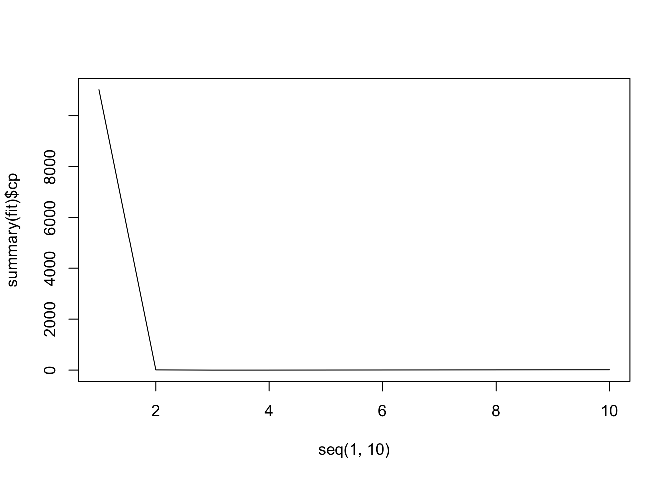
None of the studentised residuals are far outside of the (-3, 3) range, so there are no clear outliers. Some points have a leverage which exceeds 2 \times 3 / 400 = 0.015, so there are some high-levered points.
-
x <- rnorm(100)eps <- rnorm(100, 0, sqrt(0.25))y <- -1 + 0.5 * x + epsy is 100 long. \beta_0 =-1, \beta_0 = 0.5.
plot(x, y)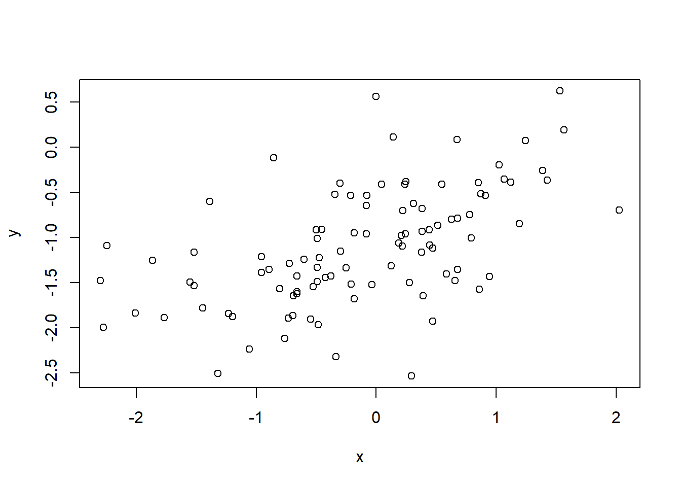
Points are approximately on an increasing straight line.
fit <- lm(y ~ x) summary(fit)Call: lm(formula = y ~ x) Residuals: Min 1Q Median 3Q Max -1.40299 -0.38140 0.02717 0.33686 1.44076 Coefficients: Estimate Std. Error t value Pr(>|t|) (Intercept) -1.04527 0.05269 -19.84 <2e-16 *** x 0.63911 0.05750 11.12 <2e-16 *** --- Signif. codes: 0 '***' 0.001 '**' 0.01 '*' 0.05 '.' 0.1 ' ' 1 Residual standard error: 0.5264 on 98 degrees of freedom Multiple R-squared: 0.5576, Adjusted R-squared: 0.5531 F-statistic: 123.5 on 1 and 98 DF, p-value: < 2.2e-16The \beta_0 estimate is within 1 standard error, and the \beta_1 estimate is within 1.1. standard errors.
plot(x, y) abline(-1, 0.5) abline(fit$coefficients[1], fit$coefficients[2], col = "red") legend("topleft", legend = c("true", "fitted"), lty = 1, col = c("black", "red") )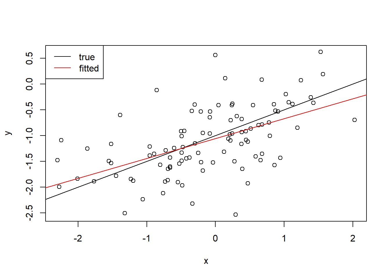
fit <- lm(y ~ x + I(x^2)) summary(fit)Call: lm(formula = y ~ x + I(x^2)) Residuals: Min 1Q Median 3Q Max -1.40928 -0.38080 0.02739 0.33155 1.44684 Coefficients: Estimate Std. Error t value Pr(>|t|) (Intercept) -1.051330 0.063422 -16.577 <2e-16 *** x 0.637794 0.058286 10.942 <2e-16 *** I(x^2) 0.007161 0.041237 0.174 0.863 --- Signif. codes: 0 '***' 0.001 '**' 0.01 '*' 0.05 '.' 0.1 ' ' 1 Residual standard error: 0.529 on 97 degrees of freedom Multiple R-squared: 0.5578, Adjusted R-squared: 0.5486 F-statistic: 61.17 on 2 and 97 DF, p-value: < 2.2e-16No. The adjusted R^2 is higher, indicating the extra term does not have significant explanatory power.
set.seed(1) x <- rnorm(100) y <- 2 * x + rnorm(100) x <- rnorm(100) eps <- rnorm(100, 0, 0.1) y <- -1 + 0.5 * x + eps fit2 <- lm(y ~ x) plot(x, y) abline(-1, 0.5) abline(fit2$coefficients[1], fit2$coefficients[2], col = "red") legend("topleft", legend = c("true", "fitted"), lty = 1, col = c("black", "red") )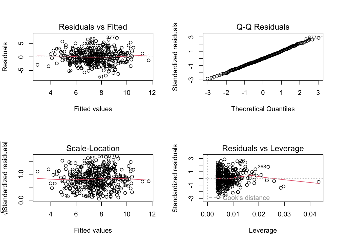
The fitted model is closer to the true model.
set.seed(1) x <- rnorm(100) y <- 2 * x + rnorm(100) x <- rnorm(100) eps <- rnorm(100, 0, 0.5) y <- -1 + 0.5 * x + eps fit3 <- lm(y ~ x) summary(fit)Call: lm(formula = y ~ x + I(x^2)) Residuals: Min 1Q Median 3Q Max -1.40928 -0.38080 0.02739 0.33155 1.44684 Coefficients: Estimate Std. Error t value Pr(>|t|) (Intercept) -1.051330 0.063422 -16.577 <2e-16 *** x 0.637794 0.058286 10.942 <2e-16 *** I(x^2) 0.007161 0.041237 0.174 0.863 --- Signif. codes: 0 '***' 0.001 '**' 0.01 '*' 0.05 '.' 0.1 ' ' 1 Residual standard error: 0.529 on 97 degrees of freedom Multiple R-squared: 0.5578, Adjusted R-squared: 0.5486 F-statistic: 61.17 on 2 and 97 DF, p-value: < 2.2e-16plot(x, y) abline(-1, 0.5) abline(fit3$coefficients[1], fit3$coefficients[2], col = "red") legend("topleft", legend = c("true", "fitted"), lty = 1, col = c("black", "red") )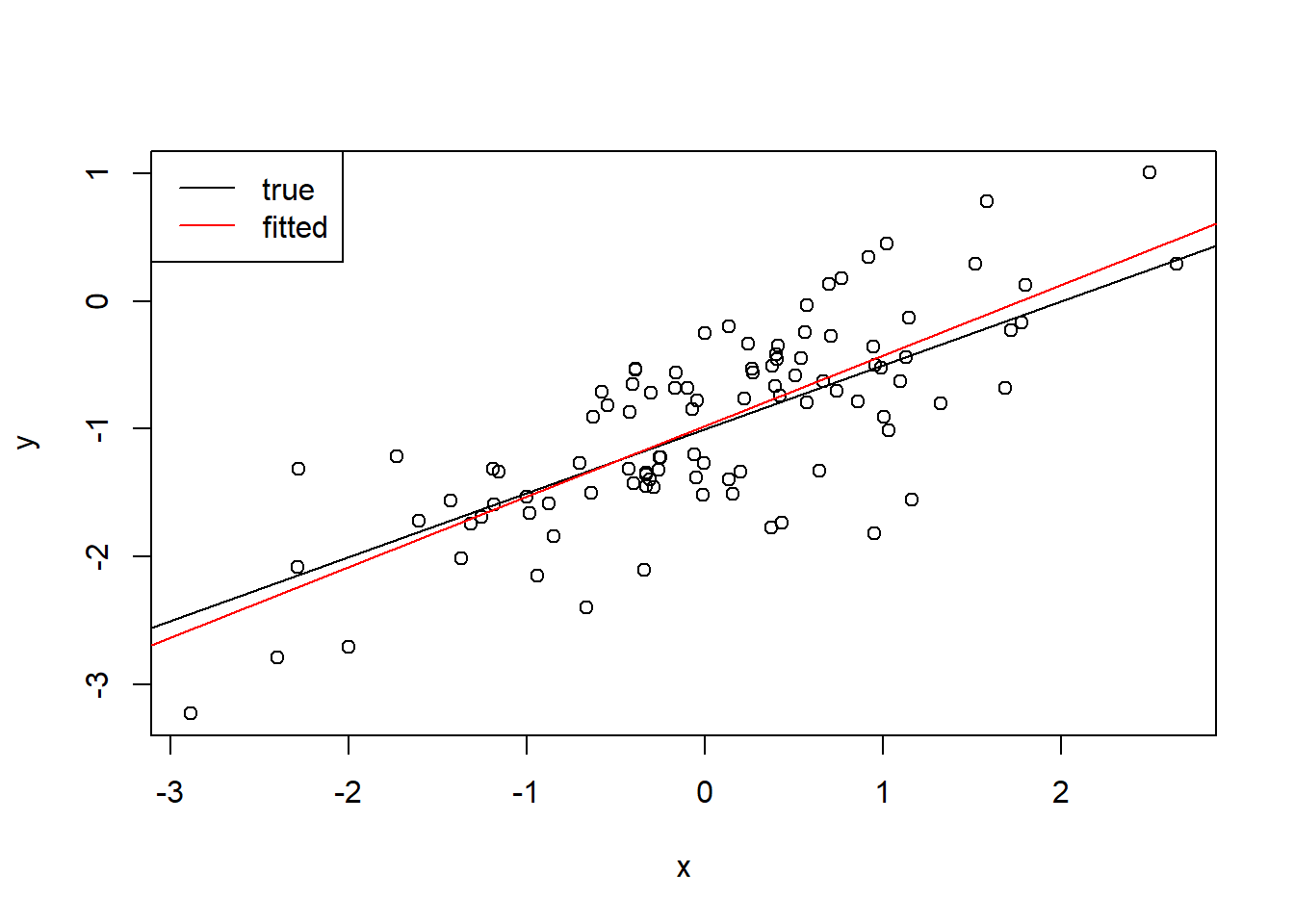
The fitted model is further away from the true model.
confint(fit) # noise=0.252.5 % 97.5 % (Intercept) -1.17720445 -0.9254556 x 0.52211261 0.7534761 I(x^2) -0.07468394 0.0890059confint(fit2) # noise=0.12.5 % 97.5 % (Intercept) -1.0148210 -0.9754890 x 0.4915195 0.5297242confint(fit3) # noise=0.52.5 % 97.5 % (Intercept) -1.0741052 -0.8774448 x 0.4575975 0.6486210The confidence interval is wider when the noise is larger.
-
\beta_0 = 2, \beta_1 = 2, \beta_2 = 0.3
set.seed(1) x1 <- runif(100) x2 <- 0.5 * x1 + rnorm(100) / 10 y <- 2 + 2 * x1 + 0.3 * x2 + rnorm(100)cor(x1, x2)[1] 0.8351212plot(x1, x2)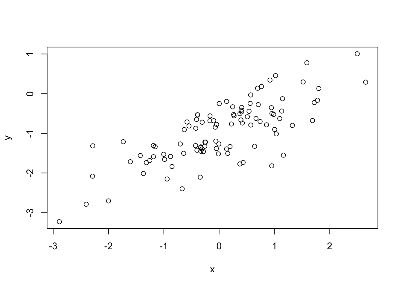
summary(lm(y ~ x1 + x2))Call: lm(formula = y ~ x1 + x2) Residuals: Min 1Q Median 3Q Max -2.8311 -0.7273 -0.0537 0.6338 2.3359 Coefficients: Estimate Std. Error t value Pr(>|t|) (Intercept) 2.1305 0.2319 9.188 7.61e-15 *** x1 1.4396 0.7212 1.996 0.0487 * x2 1.0097 1.1337 0.891 0.3754 --- Signif. codes: 0 '***' 0.001 '**' 0.01 '*' 0.05 '.' 0.1 ' ' 1 Residual standard error: 1.056 on 97 degrees of freedom Multiple R-squared: 0.2088, Adjusted R-squared: 0.1925 F-statistic: 12.8 on 2 and 97 DF, p-value: 1.164e-05The \beta_1, \beta_2 estimates are far off the true values. We can reject the null hypothesis that \beta_1 = 0 at the 95
summary(lm(y ~ x1))Call: lm(formula = y ~ x1) Residuals: Min 1Q Median 3Q Max -2.89495 -0.66874 -0.07785 0.59221 2.45560 Coefficients: Estimate Std. Error t value Pr(>|t|) (Intercept) 2.1124 0.2307 9.155 8.27e-15 *** x1 1.9759 0.3963 4.986 2.66e-06 *** --- Signif. codes: 0 '***' 0.001 '**' 0.01 '*' 0.05 '.' 0.1 ' ' 1 Residual standard error: 1.055 on 98 degrees of freedom Multiple R-squared: 0.2024, Adjusted R-squared: 0.1942 F-statistic: 24.86 on 1 and 98 DF, p-value: 2.661e-06All coefficients are significant. The estimate of \beta_0 is within 1 standard deviation of the true value. The estimate of \beta_1 is within 1 standard deviation of the true effective value.
summary(lm(y ~ x2))Call: lm(formula = y ~ x2) Residuals: Min 1Q Median 3Q Max -2.62687 -0.75156 -0.03598 0.72383 2.44890 Coefficients: Estimate Std. Error t value Pr(>|t|) (Intercept) 2.3899 0.1949 12.26 < 2e-16 *** x2 2.8996 0.6330 4.58 1.37e-05 *** --- Signif. codes: 0 '***' 0.001 '**' 0.01 '*' 0.05 '.' 0.1 ' ' 1 Residual standard error: 1.072 on 98 degrees of freedom Multiple R-squared: 0.1763, Adjusted R-squared: 0.1679 F-statistic: 20.98 on 1 and 98 DF, p-value: 1.366e-05All coefficients are significant. The estimate of \beta_0 is within 2 standard deviations of the true value. The estimate of \beta_1 is within 1 standard deviation of the true effective value.
No. Due to the collinearity, it is difficult to distinguish between the effect of x_1 and x_2 on y when they are regressed together. When regressed separately, the effect is much easier to see.
In all cases, the coefficient estimate for x_1 has decreased errantly, and that for x_2 has increased errantly. For the full model and for the x_2 only model, it is seen only has a high-leverage point. For the x_1 only model, it is seen as a high-leverage outlier.
-
set.seed(1)
X <- rnorm(100, 10, 3)
noise <- rnorm(100, 0, 2)
Y <- 4 + 3 * X + 2 * X^2 + X^3 + noisemyData <- data.frame( Y = Y, X1 = X, X2 = X^2, X3 = X^3, X4 = X^4, X5 = X^5, X6 = X^6, X7 = X^7, X8 = X^8, X9 = X^9, X10 = X^10 ) library(leaps) fit <- regsubsets(Y ~ ., data = myData, nvmax = 10) summary(fit)Subset selection object Call: regsubsets.formula(Y ~ ., data = myData, nvmax = 10) 10 Variables (and intercept) Forced in Forced out X1 FALSE FALSE X2 FALSE FALSE X3 FALSE FALSE X4 FALSE FALSE X5 FALSE FALSE X6 FALSE FALSE X7 FALSE FALSE X8 FALSE FALSE X9 FALSE FALSE X10 FALSE FALSE 1 subsets of each size up to 10 Selection Algorithm: exhaustive X1 X2 X3 X4 X5 X6 X7 X8 X9 X10 1 ( 1 ) " " " " "*" " " " " " " " " " " " " " " 2 ( 1 ) " " "*" "*" " " " " " " " " " " " " " " 3 ( 1 ) " " "*" "*" " " " " " " " " " " " " "*" 4 ( 1 ) "*" " " "*" " " "*" "*" " " " " " " " " 5 ( 1 ) " " "*" " " "*" "*" "*" "*" " " " " " " 6 ( 1 ) " " "*" "*" "*" " " " " " " "*" "*" "*" 7 ( 1 ) " " "*" " " " " "*" "*" "*" "*" "*" "*" 8 ( 1 ) " " " " "*" "*" "*" "*" "*" "*" "*" "*" 9 ( 1 ) " " "*" "*" "*" "*" "*" "*" "*" "*" "*" 10 ( 1 ) "*" "*" "*" "*" "*" "*" "*" "*" "*" "*"myData <- data.frame( Y = Y, X1 = X, X2 = X^2, X3 = X^3, X4 = X^4, X5 = X^5, X6 = X^6, X7 = X^7, X8 = X^8, X9 = X^9, X10 = X^10 ) library(leaps) fit <- regsubsets(Y ~ ., data = myData, nvmax = 10)plot(seq(1, 10), summary(fit)$cp, type = "l")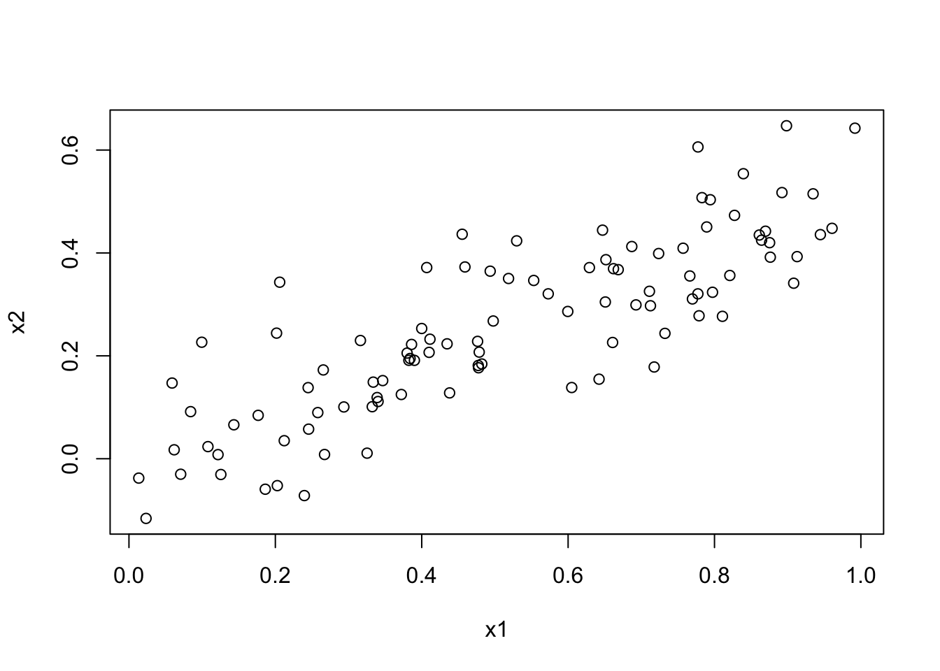
plot(seq(1, 10), summary(fit)$bic, type = "l")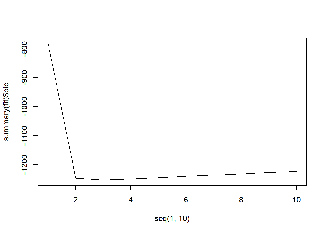
plot(seq(1, 10), summary(fit)$adjr2, type = "l")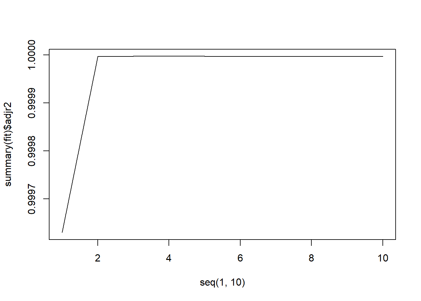
It looks like all 3 methods suggest that the 3-variable fit is the best.
summary(fit)$cp # this should give a better/clearer view[1] 11022.4698919 7.2797918 -0.6713653 0.1801732 2.1193057 [6] 4.0389022 5.9961670 7.9349196 9.7216590 11.0000000summary(fit)Subset selection object Call: regsubsets.formula(Y ~ ., data = myData, nvmax = 10) 10 Variables (and intercept) Forced in Forced out X1 FALSE FALSE X2 FALSE FALSE X3 FALSE FALSE X4 FALSE FALSE X5 FALSE FALSE X6 FALSE FALSE X7 FALSE FALSE X8 FALSE FALSE X9 FALSE FALSE X10 FALSE FALSE 1 subsets of each size up to 10 Selection Algorithm: exhaustive X1 X2 X3 X4 X5 X6 X7 X8 X9 X10 1 ( 1 ) " " " " "*" " " " " " " " " " " " " " " 2 ( 1 ) " " "*" "*" " " " " " " " " " " " " " " 3 ( 1 ) " " "*" "*" " " " " " " " " " " " " "*" 4 ( 1 ) "*" " " "*" " " "*" "*" " " " " " " " " 5 ( 1 ) " " "*" " " "*" "*" "*" "*" " " " " " " 6 ( 1 ) " " "*" "*" "*" " " " " " " "*" "*" "*" 7 ( 1 ) " " "*" " " " " "*" "*" "*" "*" "*" "*" 8 ( 1 ) " " " " "*" "*" "*" "*" "*" "*" "*" "*" 9 ( 1 ) " " "*" "*" "*" "*" "*" "*" "*" "*" "*" 10 ( 1 ) "*" "*" "*" "*" "*" "*" "*" "*" "*" "*"lm(Y ~ X2 + X3 + X10, data = myData)Call: lm(formula = Y ~ X2 + X3 + X10, data = myData) Coefficients: (Intercept) X2 X3 X10 9.871e+00 2.426e+00 9.818e-01 5.810e-12This final linear fit produces our required coefficients. We note that the model selected includes
X10instead ofX1as in the true model. However, this can be attributed to the high amount of noise in the data.Repeat the above with
method = "forward"andmethod = "backward"in theregsubsetsfunction. Alternatively, the step function can also be used here.attach(myData)The following object is masked _by_ .GlobalEnv: Ystep(lm(Y ~ 1), Y ~ X1 + X2 + X3 + X4 + X5 + X6 + X7 + X8 + X9 + X10, direction = "forward" )Start: AIC=1397.35 Y ~ 1 Df Sum of Sq RSS AIC + X3 1 114757732 42006 608.04 + X2 1 112602846 2196892 1003.74 + X4 1 111991290 2808448 1028.30 + X5 1 106159807 8639931 1140.67 + X1 1 103502796 11296942 1167.49 + X6 1 98769980 16029758 1202.48 + X7 1 90912846 23886892 1242.37 + X8 1 83280410 31519329 1270.09 + X9 1 76246003 38553735 1290.24 + X10 1 69964262 44835476 1305.33 <none> 114799738 1397.35 Step: AIC=608.04 Y ~ X3 Df Sum of Sq RSS AIC + X2 1 41623 383 140.19 + X1 1 41018 988 235.06 + X4 1 38889 3117 349.94 + X5 1 36724 5282 402.70 + X6 1 34461 7545 438.34 + X7 1 32254 9752 464.01 + X8 1 30178 11828 483.30 + X9 1 28269 13737 498.27 + X10 1 26537 15469 510.14 <none> 42006 608.04 Step: AIC=140.19 Y ~ X3 + X2 Df Sum of Sq RSS AIC + X10 1 37.596 345.04 131.85 + X9 1 37.224 345.41 131.96 + X8 1 36.673 345.96 132.12 + X7 1 35.924 346.71 132.33 + X6 1 34.960 347.68 132.61 + X5 1 33.771 348.87 132.95 + X4 1 32.355 350.28 133.36 + X1 1 26.801 355.84 134.93 <none> 382.64 140.19 Step: AIC=131.85 Y ~ X3 + X2 + X10 Df Sum of Sq RSS AIC <none> 345.04 131.85 + X9 1 0.234893 344.81 133.78 + X1 1 0.201465 344.84 133.79 + X8 1 0.194667 344.85 133.79 + X7 1 0.145658 344.90 133.81 + X6 1 0.091731 344.95 133.82 + X5 1 0.040675 345.00 133.84 + X4 1 0.005680 345.04 133.85Call: lm(formula = Y ~ X3 + X2 + X10) Coefficients: (Intercept) X3 X2 X10 9.871e+00 9.818e-01 2.426e+00 5.810e-12step(lm(Y ~ X1 + X2 + X3 + X4 + X5 + X6 + X7 + X8 + X9 + X10), Y ~ ., direction = "backward" )Start: AIC=143.27 Y ~ X1 + X2 + X3 + X4 + X5 + X6 + X7 + X8 + X9 + X10 Df Sum of Sq RSS AIC - X1 1 2.7265 338.97 142.07 - X2 1 2.8364 339.08 142.11 - X3 1 2.9696 339.21 142.15 - X4 1 3.0773 339.32 142.18 - X5 1 3.1874 339.43 142.21 - X6 1 3.2898 339.53 142.24 - X7 1 3.3841 339.63 142.27 - X8 1 3.4702 339.71 142.29 - X9 1 3.5485 339.79 142.32 - X10 1 3.6194 339.86 142.34 <none> 336.24 143.27 Step: AIC=142.07 Y ~ X2 + X3 + X4 + X5 + X6 + X7 + X8 + X9 + X10 Df Sum of Sq RSS AIC - X2 1 0.80571 339.78 140.31 - X4 1 1.02949 340.00 140.38 - X3 1 1.03604 340.01 140.38 - X5 1 1.07147 340.04 140.39 - X6 1 1.10354 340.07 140.40 - X7 1 1.12948 340.10 140.41 - X8 1 1.15180 340.12 140.41 - X9 1 1.17205 340.14 140.42 - X10 1 1.19094 340.16 140.43 <none> 338.97 142.07 Step: AIC=140.31 Y ~ X3 + X4 + X5 + X6 + X7 + X8 + X9 + X10 Df Sum of Sq RSS AIC - X10 1 0.5185 340.30 138.46 - X9 1 0.5352 340.31 138.47 - X8 1 0.5652 340.34 138.48 - X7 1 0.6169 340.39 138.49 - X6 1 0.7065 340.48 138.52 - X5 1 0.8712 340.65 138.57 - X4 1 1.2277 341.00 138.67 - X3 1 4.5218 344.30 139.63 <none> 339.78 140.31 Step: AIC=138.46 Y ~ X3 + X4 + X5 + X6 + X7 + X8 + X9 Df Sum of Sq RSS AIC - X9 1 0.1097 340.41 136.50 - X8 1 0.2031 340.50 136.52 - X7 1 0.3659 340.66 136.57 - X6 1 0.6572 340.95 136.66 - X5 1 1.2250 341.52 136.82 - X4 1 2.5848 342.88 137.22 <none> 340.30 138.46 - X3 1 21.8581 362.15 142.69 Step: AIC=136.5 Y ~ X3 + X4 + X5 + X6 + X7 + X8 Df Sum of Sq RSS AIC <none> 340.41 136.50 - X8 1 7.536 347.94 136.69 - X7 1 9.306 349.71 137.19 - X6 1 11.903 352.31 137.93 - X5 1 16.360 356.76 139.19 - X4 1 26.328 366.73 141.95 - X3 1 193.910 534.32 179.58Call: lm(formula = Y ~ X3 + X4 + X5 + X6 + X7 + X8) Coefficients: (Intercept) X3 X4 X5 X6 X7 1.157e+01 2.389e+00 -3.353e-01 4.141e-02 -2.789e-03 9.721e-05 X8 -1.372e-06Note that the forward direction gives the same model as best-subset selection but the backward direction gives a different model!
For ease, just set the following and rerun the above code.
myData["Y"] <- 10 + 2 * X^7 + noiseIn this case, it seems that the best-subset algorithm produces the best model to be the 3-predictor model, with
X6,X7andX8as predictors. Lasso would force some predictors to zero but still retain 5 predictors and so is not doing well in this case.