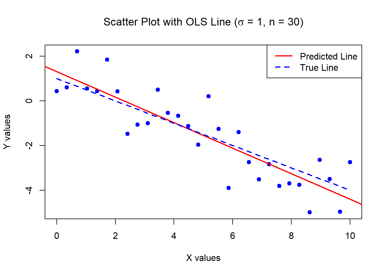
Estimates of Beta_0 and Beta_1:
 1.309629 -0.5713465
Standard error of the estimates:
0.346858 0.05956626 Some of the figures in this presentation are taken from “An Introduction to Statistical Learning, with applications in R” (Springer, 2013) with permission from the authors: G. James, D. Witten, T. Hastie and R. Tibshirani
James et al. (2021), Chapter 3, Chapter 6.1
Suppose we have pairs of data (y_1, x_1), (y_2, x_2), ..., (y_n, x_n) and we want to predict values of y_i based on x_i.
These are all examples of “models” we can specify. Let’s focus on the linear prediction. Some questions:
In simple linear regression, we predict that a quantitive response “Y” is a linear function of a single predictor “X”, Y \approx \beta_0 + \beta_1 X.
“Simple” here refers to the fact there is a single predictor.
Assume we have n observations, and call \bm{y} = (y_1, ..., y_n)^\top the vector of responses and \bm{x} = (x_1,...,x_n)^{\top} the vector of correpsonding predictors. Our model states that the ‘true’ relationship between X and Y is linear (plus a “noise” or “error”). Using vector notation, we write: \bm{y} = \beta_0 + \beta_1 \bm{x} + \bm{\epsilon},
where \bm{\epsilon} = (\epsilon_1, ..., \epsilon_n)^{\top} is a vector of error terms (respecting certain assumptions).
Advertising Example\texttt{sales} \approx \beta_0 + \beta_1 \times \texttt{TV}
Weak assumptions \mathbb{E}( \epsilon_i|\bm{x}) = 0,\quad \mathbb{V}( \epsilon_i|\bm{x}) = \sigma^2 \text{and}\quad Cov(\epsilon_i,\epsilon_j|\bm{x})=0 for i=1,2,3,...,n; for all i \neq j.
In other words, errors have zero mean, common variance and are conditionally uncorrelated. Those are the minimum assumptions for “Least Squares” estimation.
Strong assumptions \epsilon_i|\bm{x} \overset{\text{i.i.d.}}{\sim} \mathcal{N}(0,\sigma^2) for i=1,2,3,...,n. In other words, errors are i.i.d. Normal random variables with zero mean and constant variance. Those are the minimum assumptions for “Maximum Likelihood” estimation.
Recall we assume the ‘true’ relationship between X and Y (seen here as random variables) is described by Y =\beta_0 + \beta_1 X + \epsilon, where \epsilon satisfies either the weak or strong assumptions.
If we have an observed sample from (X,Y), say (x_1, y_1), ..., (x_n, y_n), we then want to obtain estimates \hat{\beta}_0 and \hat{\beta}_1 of the parameters \beta_0, \beta_1.
Once we have these estimates, we can predict any “response” simply by: \hat{y}_i=\hat{\beta}_0 + \hat{\beta}_1 x_i.
This makes sense because \begin{aligned} \mathbb{E}[Y|X=x_i] & = \mathbb{E}[\beta_0 + \beta_1 X + \epsilon_i | X=x_i] = {\beta}_0 + {\beta}_1 x_i \end{aligned} (where we used the fact that \mathbb{E}[\epsilon_i|X=x_i] = 0).
Under the weak assumptions we have that the (co-)variances of the parameters are: \begin{aligned} \text{Var}\left(\hat{\beta }_{0}|\bm{x}\right) =&\sigma^2\left(\frac{1}{n}+\frac{\overline{x}^2}{\sum_{i=1}^{n}(x_i-\overline{x})^2}\right)=\sigma^2\left(\frac{1}{n}+\frac{\overline{x}^2}{S_{xx}}\right)\\{ }=& SE(\hat{\beta_0})^2\\ \text{Var}\left( \hat{\beta }_{1}|\bm{x}\right) =& \frac{\sigma^2}{\sum_{i=1}^{n}(x_i-\overline{x})^2}=\frac{\sigma^2}{S_{xx}}=SE(\hat{\beta_1})^2\\ %= \frac{n\sigma^2}{nS_{xx}-S_{x}^2}\\ \text{Cov}\left( \hat{\beta }_{0},\hat{\beta }_{1}|\bm{x}\right) =& -\frac{ \overline{x} \sigma^2}{\sum_{i=1}^{n}(x_i-\overline{x})^2}=-\frac{ \overline{x} \sigma^2}{S_{xx}} %%s_\epsilon^2 = \text{Var}\left(\hat{\epsilon}\right) =& \frac{nS_{yy}-S_y^2-\hat{\beta}_1^2(nS_{xx}-S_x^2)}{n(n-2)} \end{aligned}
Proof: See Lab questions. Hopefully you can see that all three quantities go to 0 as n gets larger.
Proof: Since Y_i|x_i = \beta_0 + \beta_1 x_i + \epsilon_i, where \epsilon_i \overset{\text{i.i.d.}}{\sim} \mathcal{N}(0,\sigma^2), then Y_i|x_i \overset{\text{i.i.d.}}{\sim} \mathcal{N}\left( \beta_0 + \beta_1 x_i, \sigma^2 \right). The result follows.
Partial derivatives set to zero give the following MLEs: \begin{aligned} \hat{\beta}_1=&\frac{\sum_{i=1}^{n}\left( x_{i}-\overline{x}\right) \left( y_{i}-\overline{y}\right) }{\sum_{i=1}^{n}\left( x_{i}-\overline{x}\right) ^{2}}=\frac{S_{xy}}{S_{xx}},\\ \hat{\beta}_0=&\overline{y}-\hat{\beta}_1\overline{x}, \end{aligned} and \hat{\sigma }_{\text{MLE}}^{2}=\frac{1}{n}\sum_{i=1}^{n}\left( y_{i}-\left( \hat{\beta}_0+\hat{\beta}_1x_{i}\right) \right) ^{2}.
How do we interpret a linear regression model such as \hat{\beta}_0 = 1 and \hat{\beta}_1 = -0.5?
The below data was generated by Y = 1 - 0.5\times X + \epsilon where X \sim U[0,10] and \epsilon \sim N(0,1) with n = 30.

Estimates of Beta_0 and Beta_1:
1.309629 -0.5713465 Standard error of the estimates:
0.346858 0.05956626 The below data was generated by Y = 1 - 0.5\times X + \epsilon where X \sim U[0,10] and \epsilon \sim N(0,1) with n = 5000.
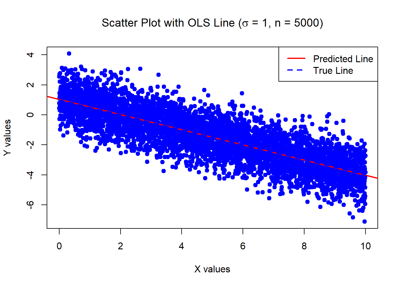
Estimates of Beta_0 and Beta_1:
 1.028116 -0.5057372
Standard error of the estimates:
0.02812541 0.00487122 The below data was generated by Y = 1 - 0.5\times X + \epsilon where X \sim U[0,10] and \epsilon \sim N(0, \sigma^2=100) with n = 30.

Estimates of Beta_0 and Beta_1:
 -2.19991 -0.4528679
Standard error of the estimates:
3.272989 0.5620736 The below data was generated by Y = 1 - 0.5\times X + \epsilon where X \sim U[0,10] and \epsilon \sim N(0, \sigma^2=100) with n = 5000.
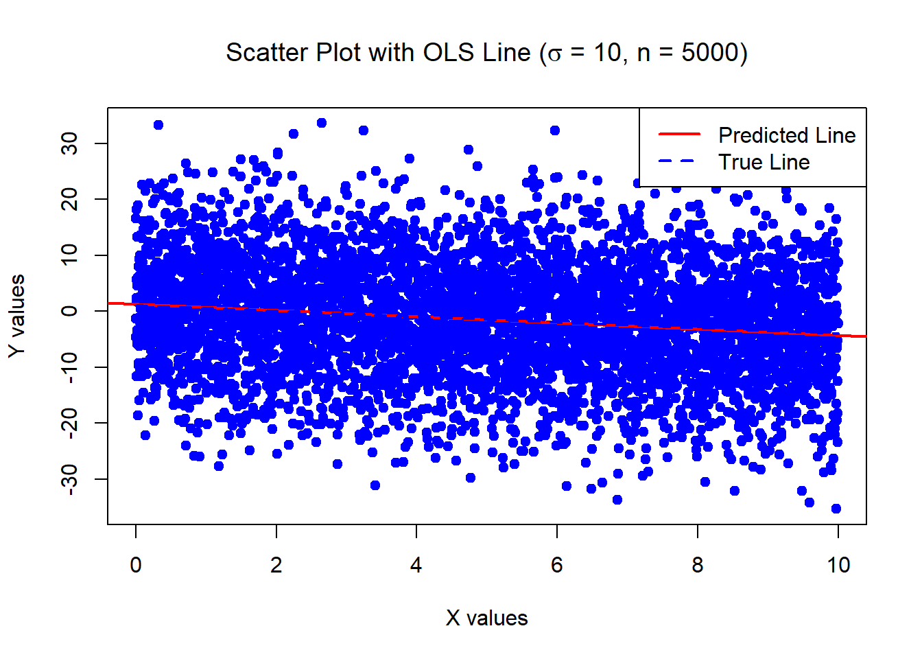
Estimates of Beta_0 and Beta_1:
 1.281162 -0.5573716
Standard error of the estimates:
0.2812541 0.0487122 The below data was generated by Y = 1 - 40\times X + \epsilon where X \sim U[0,10] and \epsilon \sim N(0,100) with n = 30.
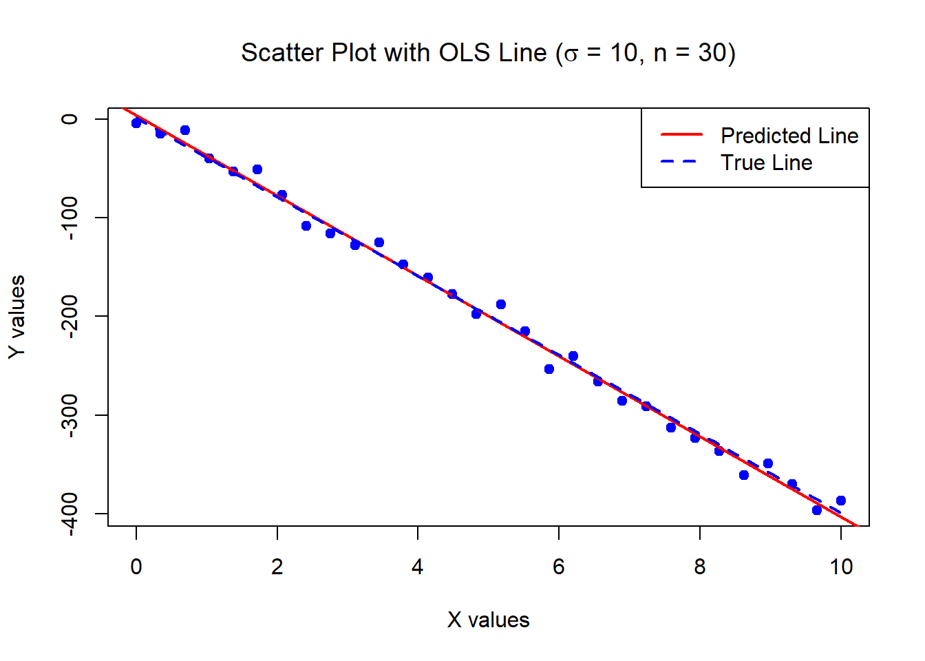
Estimates of Beta_0 and Beta_1:
 4.096286 -40.71346
Standard error of the estimates:
3.46858 0.5956626 The below data was generated by Y = 1 + 0.2 \times X^2 + \epsilon where X \sim U[0,10] and \epsilon \sim N(0, \sigma^2=0.01) with n = 500.

Estimates of Beta_0 and Beta_1:
 -2.32809 2.000979
Variances of the estimates:
0.01808525 0.0005420144 For inference (e.g., confidence intervals, hypothesis tests), we need the strong assumptions!
Using the strong assumptions, 100\left( 1-\alpha \right) \% confidence intervals (CI) for \beta_1 and \beta_0 are given by:
\hat{\beta}_1\pm t_{1-\alpha /2,n-2}\cdot \underbrace{\dfrac{s}{\sqrt{S_{xx}}}}_{\hat{SE}(\hat{\beta}_1)}
\hat{\beta}_0\pm t_{1-\alpha /2,n-2}\cdot \underbrace{s\sqrt{\frac{1}{n}+\frac{\overline{x}^2}{S_{xx}}}}_{\hat{SE}(\hat{\beta}_0)}
See rationale slide.
We can test whether the predictor has any influence on the response (or if the influence is larger/smaller than some value).
For testing the hypothesis H_{0}:\beta_1 =\widetilde{\beta}_1 \quad\text{vs}\quad H_{1}:\beta_1 \neq \widetilde{\beta}_1, (where \widetilde{\beta}_1 is any constant) we use the test statistic: t(\hat{\beta}_1) = \dfrac{\hat{\beta}_1-\widetilde{\beta}_1}{\hat{SE}(\hat{\beta_1})}=\dfrac{\hat{\beta}_1-\widetilde{\beta}_1}{\left( s\left/ \sqrt{S_{xx}}\right. \right)} which has a t_{n-2} distribution under H_0 (see rationale slide).
The construction of the hypothesis test is the same for \beta_0.
The decision rules under various alternative hypotheses are summarized below.
| Alternative H_{1} | Reject H_{0} in favor of H_{1} if |
|---|---|
| \beta_1 \neq \widetilde{\beta}_1 | \left\vert t\left( \hat{\beta}_1\right) \right\vert >t_{1-\alpha /2,n-2} |
| \beta_1 >\widetilde{\beta}_1 | t\left( \hat{\beta}_1\right)>t_{1-\alpha ,n-2} |
| \beta_1 <\widetilde{\beta}_1 | t\left( \hat{\beta}_1\right)<-t_{1-\alpha ,n-2} |
The below data was generated by Y = 1 - 0.5\times X + \epsilon where X \sim U[0,10] and \epsilon \sim N(0,1) with n = 30.
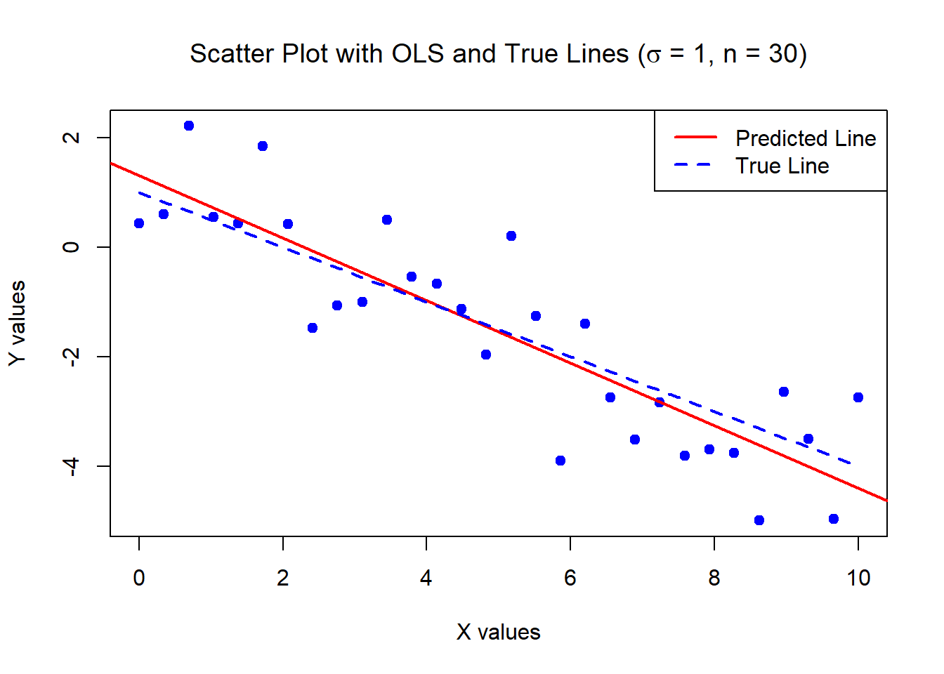
Call:
lm(formula = Y ~ X)

Residuals:
    Min      1Q  Median      3Q     Max
-1.8580 -0.7026 -0.1236  0.5634  1.8463

Coefficients:
            Estimate Std. Error t value Pr(>|t|)
(Intercept)  1.30963    0.34686   3.776 0.000764 ***
X           -0.57135    0.05957  -9.592  2.4e-10 ***
---
Signif. codes:  0 '***' 0.001 '**' 0.01 '*' 0.05 '.' 0.1 ' ' 1

Residual standard error: 0.9738 on 28 degrees of freedom
Multiple R-squared:  0.7667,    Adjusted R-squared:  0.7583
F-statistic: 92 on 1 and 28 DF, p-value: 2.396e-10The below data was generated by Y = 1 - 0.5\times X + \epsilon where X \sim U[0,10] and \epsilon \sim N(0,1) with n = 5000.

Call:
lm(formula = Y ~ X)

Residuals:
    Min      1Q  Median      3Q     Max
-3.1179 -0.6551 -0.0087  0.6655  3.4684

Coefficients:
             Estimate Std. Error t value Pr(>|t|)
(Intercept)  1.028116   0.028125   36.55   <2e-16 ***
X           -0.505737   0.004871 -103.82   <2e-16 ***
---
Signif. codes:  0 '***' 0.001 '**' 0.01 '*' 0.05 '.' 0.1 ' ' 1

Residual standard error: 0.9945 on 4998 degrees of freedom
Multiple R-squared:  0.6832,    Adjusted R-squared:  0.6831
F-statistic: 1.078e+04 on 1 and 4998 DF, p-value: < 2.2e-16The below data was generated by Y = 1 - 0.5\times X + \epsilon where X \sim U[0,10] and \epsilon \sim N(0,100) with n = 30.
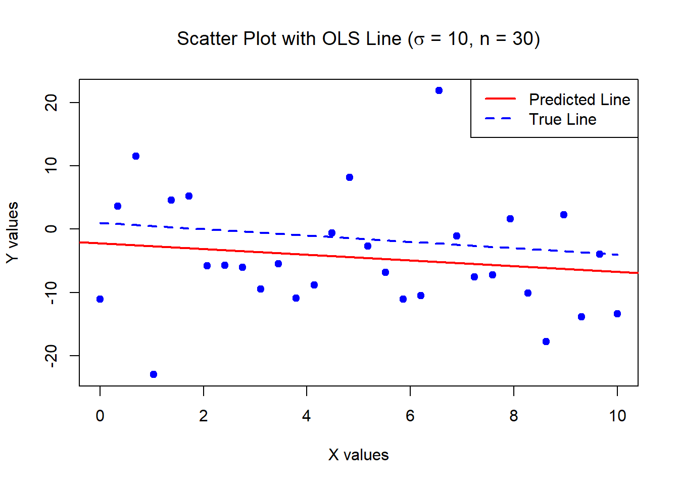
Call:
lm(formula = Y ~ X)

Residuals:
    Min      1Q  Median      3Q     Max
-20.306  -5.751  -2.109   5.522  27.049

Coefficients:
            Estimate Std. Error t value Pr(>|t|)
(Intercept)  -2.1999     3.2730  -0.672    0.507
X            -0.4529     0.5621  -0.806    0.427

Residual standard error: 9.189 on 28 degrees of freedom
Multiple R-squared:  0.02266,   Adjusted R-squared:  -0.01225
F-statistic: 0.6492 on 1 and 28 DF, p-value: 0.4272The below data was generated by Y = 1 - 0.5\times X + \epsilon where X \sim U[0,10] and \epsilon \sim N(0,100) with n = 5000.

Call:
lm(formula = Y ~ X)

Residuals:
    Min      1Q  Median      3Q     Max
-31.179  -6.551  -0.087   6.655  34.684

Coefficients:
            Estimate Std. Error t value Pr(>|t|)
(Intercept)  1.28116    0.28125   4.555 5.36e-06 ***
X           -0.55737    0.04871 -11.442  < 2e-16 ***
---
Signif. codes:  0 '***' 0.001 '**' 0.01 '*' 0.05 '.' 0.1 ' ' 1

Residual standard error: 9.945 on 4998 degrees of freedom
Multiple R-squared:  0.02553,   Adjusted R-squared:  0.02533
F-statistic: 130.9 on 1 and 4998 DF, p-value: < 2.2e-16The below data was generated by Y = 1 - 40\times X + \epsilon where X \sim U[0,10] and \epsilon \sim N(0,100) with n = 30.
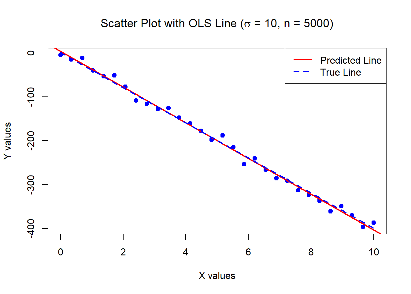
Call:
lm(formula = Y ~ X)

Residuals:
    Min      1Q  Median      3Q     Max
-18.580  -7.026  -1.236   5.634  18.463

Coefficients:
            Estimate Std. Error t value Pr(>|t|)
(Intercept)   4.0963     3.4686   1.181    0.248
X           -40.7135     0.5957 -68.350   <2e-16 ***
---
Signif. codes:  0 '***' 0.001 '**' 0.01 '*' 0.05 '.' 0.1 ' ' 1

Residual standard error: 9.738 on 28 degrees of freedom
Multiple R-squared:  0.994, Adjusted R-squared:  0.9938
F-statistic: 4672 on 1 and 28 DF, p-value: < 2.2e-16The below data was generated by Y = 1 + 0.2 \times X^2 + \epsilon where X \sim U[0,10] and \epsilon \sim N(0,0.01) with n = 500.
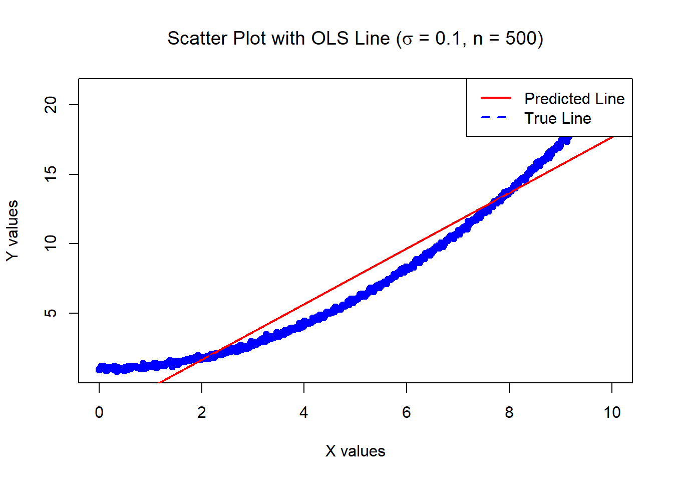
Call:
lm(formula = Y ~ X)

Residuals:
    Min      1Q  Median      3Q     Max
-1.8282 -1.3467 -0.4217  1.1207  3.4041

Coefficients:
            Estimate Std. Error t value Pr(>|t|)
(Intercept) -2.32809    0.13448  -17.31   <2e-16 ***
X            2.00098    0.02328   85.95   <2e-16 ***
---
Signif. codes:  0 '***' 0.001 '**' 0.01 '*' 0.05 '.' 0.1 ' ' 1

Residual standard error: 1.506 on 498 degrees of freedom
Multiple R-squared:  0.9368,    Adjusted R-squared:  0.9367
F-statistic: 7387 on 1 and 498 DF, p-value: < 2.2e-16Below is the summary of the hypothesis tests for whether the \beta_j are statistically different from 0 for the six examples, at a 5% level.
| 1 | 2 | 3 | 4 | 5 | 6 | |
|---|---|---|---|---|---|---|
| \beta_0 | Y | Y | N | Y | N | Y |
| \beta_1 | Y | Y | N | Y | Y | Y |
Does that mean the models that are significant at 5% for both \beta_0 and \beta_1 are equivalently ‘good’ models?
We have the following so far:
We now discuss how to assess whether a model is ‘good’ / ‘accurate’?
Partitioning the variability is used to assess how well the linear model explains the trend in data:
\underset{\text{total deviation}}{\underbrace{y_{i}-\overline{y}}}=\underset{\text{unexplained deviation}}{\underbrace{\left( y_{i}-\hat{y}_{i}\right) }}+\underset{\text{explained deviation}}{\underbrace{\left( \hat{y}_{i}-\overline{y}\right). }}
We can show (see Lab questions) that :
\underset{\text{TSS}}{\underbrace{\overset{n}{\underset{i=1}{\sum }}\left( y_{i}-\overline{y}\right) ^{2}}}=\underset{\text{RSS}}{\underbrace{\overset{n}{\underset{i=1}{\sum }}\left( y_{i}-\hat{y}_{i}\right) ^{2}}}+\underset{\text{MSS}}{\underbrace{\overset{n}{\underset{i=1}{\sum }}\left( \hat{y}_{i}-\overline{y}\right) ^{2}}},
How to interpret these sums of squares:
This partitioning of the variability is used in “ANOVA tables”:
| Source | Sum of squares | DoF | Mean squares | F-stat |
|---|---|---|---|---|
| Regression | \text{MSS}= \sum_{i=1}^{n} (\hat{y_i} - \bar{y})^2 | \text{DFM} = 1 | \frac{\text{MSS}}{\text{DFM}} | \frac{\text{MSS}/\text{DFM}}{\text{RSS}/\text{DFE}} |
| Error | \text{RSS}= \sum_{i=1}^{n} (y_i - \hat{y_i})^2 | \text{DFE} = n-2 | \frac{\text{RSS}}{\text{DFE}} | |
| Total | \text{TSS} = \sum_{i=1}^{n} (y_i - \bar{y})^2 | \text{DFT} = n-1 | \frac{\text{TSS}}{\text{DFT}} |
R^2 = \frac{\text{MSS}}{\text{TSS}} = 1 - \frac{\text{RSS}}{\text{TSS}}.
Below is a table of the R^2 for all of the six examples:
| 1 | 2 | 3 | 4 | 5 | 6 | |
|---|---|---|---|---|---|---|
| R^2 | 0.77 | 0.68 | 0.02 | 0.03 | 0.99 | 0.94 |
Advertising Example\texttt{sales} \approx \beta_0 + \beta_1 \times \texttt{TV}+ \beta_2 \times \texttt{radio}
\bm{X}=\left[ \begin{array}{ccccc} 1 & x_{11} & x_{12} & \ldots & x_{1p} \\ 1 & x_{21} & x_{22} & \ldots & x_{2p} \\ \vdots & \vdots & \vdots & \ddots & \vdots \\ 1 & x_{n1} & x_{n2} & \ldots & x_{np} \end{array} \right]
The asssumptions made about the errors are as in simple linear regression:
The error terms \epsilon_{i} satisfy the following: \begin{aligned} \begin{array}{rll} \mathbb{E}[ \epsilon _{i}|\bm{X}] =&0, &\text{ for }i=1,2,\ldots,n; \\ \text{Var}( \epsilon _{i}|\bm{X}) =&\sigma ^{2}, &\text{ for }i=1,2,\ldots,n;\\ \text{Cov}( \epsilon _{i},\epsilon _{j}|\bm{X})=&0, &\text{ for all }i\neq j. \end{array} \end{aligned}
In words, the errors have zero means, common variance, and are uncorrelated. In matrix form, we have: \begin{aligned} \mathbb{E}\left[ \bm{\epsilon} | \bm{X}\right] = \bm{0}; \qquad \text{Cov}\left( \bm{\epsilon} | \bm{X} \right) =\sigma^{2} I_n, \end{aligned} where I_n is the n\times n identity matrix.
Under the weak assumptions we have unbiased estimators:
One (usually bad) solution: assign a number to each categorical value.
Problem? The numbers you use specify a relationship between the categories. For example, we are saying a Bachelors degree is above a HS diploma (in particular, it is worth exactly 2x more). So, \beta_{edu} (B) = 2 \times \beta_{edu} (HS).
In some contexts, it might make some sense, but in general it seems unnecessarily restrictive.
And if the categories are completely unrelated (no natural ordering makes sense, e.g., colors), this approach won’t work at all.
\begin{pmatrix} R \\ G \\ G \\ B \\ \end{pmatrix} = \begin{pmatrix} 1 & 0 & 0 \\ 0 & 1 & 0 \\ 0 & 1 & 0 \\ 0 & 0 & 1 \\ \end{pmatrix}, where the first column represents red, second green and third blue.
\begin{pmatrix} R \\ G \\ G \\ B \\ \end{pmatrix} = \begin{pmatrix} 0 & 0 \\ 1 & 0 \\ 1 & 0 \\ 0 & 1 \\ \end{pmatrix}, where the first column is an indicator for “green”, second for “blue”. If both values are 0 for a given observation (i.e., a given row), this observation is ‘Red’.
| TV | radio | sales |
|---|---|---|
| 230.1 | 37.8 | 22.1 |
| 44.5 | 39.3 | 10.4 |
| 17.2 | 45.9 | 9.3 |
| 151.5 | 41.3 | 18.5 |
| 180.8 | 10.8 | 12.9 |
| 8.7 | 48.9 | 7.2 |
| 57.5 | 32.8 | 11.8 |
| 120.2 | 19.6 | 13.2 |
| 8.6 | 2.1 | 4.8 |
| 199.8 | 2.6 | 10.6 |
| 66.1 | 5.8 | 8.6 |
\bm{y} = \bm{X} \bm{\beta} + \bm{\epsilon} \bm{X} = \left[ \begin{array}{ccccc} 1 & x_{11} & x_{12} & \ldots & x_{1p} \\ 1 & x_{21} & x_{22} & \ldots & x_{2p} \\ \vdots & \vdots & \vdots & \ddots & \vdots \\ 1 & x_{n1} & x_{n2} & \ldots & x_{np} \end{array} \right] \bm{\beta} = \left[ \begin{array}{c} \beta_{0} \\ % \beta_{1} \\ \vdots \\ \beta_{p} \end{array} \right] \bm{y} = \left[ \begin{array}{c} y_{1} \\ y_{2} \\ \vdots \\ y_{n} \end{array} \right]
library(tidyverse)
site <- url("https://www.statlearning.com/s/Advertising.csv")
df_adv <- read_csv(site, show_col_types = FALSE)
X <- model.matrix(~ TV + radio, data = df_adv);
y <- df_adv[, "sales"]head(X) (Intercept) TV radio
1 1 230.1 37.8
2 1 44.5 39.3
3 1 17.2 45.9
4 1 151.5 41.3
5 1 180.8 10.8
6 1 8.7 48.9head(y)# A tibble: 6 × 1
sales
<dbl>
1 22.1
2 10.4
3 9.3
4 18.5
5 12.9
6 7.2lm and predict\hat{\bm{\beta}} = (\bm{X}^\top\bm{X})^{-1} \bm{X}^\top \bm{y}
model <- lm(sales ~ TV + radio, data = df_adv)
coef(model)
(Intercept) TV radio
2.92109991 0.04575482 0.18799423 X <- model.matrix(~ TV + radio, data = df_adv)
y <- df_adv$sales
beta <- solve(t(X) %*% X) %*% t(X) %*% y
beta [,1]
(Intercept) 2.92109991
TV 0.04575482
radio 0.18799423\hat{\bm{y}} = \bm{X} \hat{\bm{\beta}}.
budgets <- data.frame(TV = c(100, 200, 300), radio = c(20, 30, 40))
predict(model, newdata = budgets)
1 2 3
11.25647 17.71189 24.16731 X_new <- model.matrix(~ TV + radio, data = budgets)
X_new %*% beta [,1]
1 11.25647
2 17.71189
3 24.16731Design matrices are normally an ‘Excel’-style table of covariates/predictors plus a column of ones.
If categorical variables are present, they are added as dummy variables:
fake <- tibble(
  speed = c(100, 80, 60, 60, 120, 40),
  risk = c("Low", "Medium", "High",
           "Medium", "Low", "Low")
)
fake
# A tibble: 6 × 2
speed risk
<dbl> <chr>
1 100 Low
2 80 Medium
3 60 High
4 60 Medium
5 120 Low
6 40 Low model.matrix(~ speed + risk, data = fake) (Intercept) speed riskLow riskMedium
1 1 100 1 0
2 1 80 0 1
3 1 60 0 0
4 1 60 0 1
5 1 120 1 0
6 1 40 1 0
attr(,"assign")
[1] 0 1 2 2
attr(,"contrasts")
attr(,"contrasts")$risk
[1] "contr.treatment"What happens if we don’t drop the last level of the dummy variables ?
X_dummy = model.matrix(~ risk, data = fake)
as.data.frame(X_dummy)
(Intercept) riskLow riskMedium
1 1 1 0
2 1 0 1
3 1 0 0
4 1 0 1
5 1 1 0
6 1 1 0solve(t(X_dummy) %*% X_dummy) (Intercept) riskLow riskMedium
(Intercept) 1 -1.000000 -1.0
riskLow -1 1.333333 1.0
riskMedium -1 1.000000 1.5X_oh <- cbind(X_dummy, riskHigh = (fake$risk == "High"))
as.data.frame(X_oh) (Intercept) riskLow riskMedium riskHigh
1 1 1 0 0
2 1 0 1 0
3 1 0 0 1
4 1 0 1 0
5 1 1 0 0
6 1 1 0 0solve(t(X_oh) %*% X_oh)Error in solve.default(t(X_oh) %*% X_oh): system is computationally singular: reciprocal condition number = 6.93889e-18| Source | Sum of squares | DoF | Mean squares | F-stat |
|---|---|---|---|---|
| Regression | \text{MSS}= \sum_{i=1}^{n} (\hat{y_i} - \bar{y})^2 | \text{DFM} = p | \frac{\text{MSS}}{\text{DFM}} | \frac{\text{MSS}/\text{DFM}}{\text{RSS}/\text{DFE}} |
| Error | \text{RSS}= \sum_{i=1}^{n} (y_i - \hat{y_i})^2 | \text{DFE} = n-p-1 | \frac{\text{RSS}}{\text{DFE}} | |
| Total | \text{TSS} = \sum_{i=1}^{n} (y_i - \bar{y})^2 | \text{DFT} = n-1 | \frac{\text{TSS}}{\text{DFT}} |
H_0: \beta_1 = \cdots = \beta_p = 0 \quad \text{vs} \quad H_a: \text{at least one } \beta_j \text{ is non-zero}
Advertising Example (continued)Linear regression fit using TV and Radio:
What do you observe?
The below data was generated by Y = 1 - 0.7\times X_1 + X_2 + \epsilon where X_1, X_2 \sim U[0,10] and \epsilon \sim N(0,1) with n = 30.
The below data was generated by Y = 1 - 0.7\times X_1 + X_2 + \epsilon where X_1, X_2 \sim U[0,10] and \epsilon \sim N(0,1) with n = 30.
Call:
lm(formula = Y ~ X1 + X2)

Residuals:
    Min      1Q  Median      3Q     Max
-1.6923 -0.4883 -0.1590  0.5366  1.9996

Coefficients:
            Estimate Std. Error t value Pr(>|t|)
(Intercept)  1.22651    0.45843   2.675   0.0125 *
X1          -0.71826    0.05562 -12.913 4.56e-13 ***
X2           1.01285    0.05589  18.121  < 2e-16 ***
---
Signif. codes:  0 '***' 0.001 '**' 0.01 '*' 0.05 '.' 0.1 ' ' 1

Residual standard error: 0.8625 on 27 degrees of freedom
Multiple R-squared:  0.9555,    Adjusted R-squared:  0.9522
F-statistic: 290.1 on 2 and 27 DF, p-value: < 2.2e-16The below data was generated by Y = 1 - 0.7\times X_1 + X_2 + \epsilon where X_1, X_2 \sim U[0,10] and \epsilon \sim N(0, \sigma^2=100) with n = 30.
The below data was generated by Y = 1 - 0.7\times X_1 + X_2 + \epsilon where X_1, X_2 \sim U[0,10] and \epsilon \sim N(0,100) with n = 30.
Call:
lm(formula = Y ~ X1 + X2)

Residuals:
    Min      1Q  Median      3Q     Max
-16.923  -4.883  -1.591   5.366  19.996

Coefficients:
            Estimate Std. Error t value Pr(>|t|)
(Intercept)   3.2651     4.5843   0.712   0.4824
X1           -0.8826     0.5562  -1.587   0.1242
X2            1.1285     0.5589   2.019   0.0535 .
---
Signif. codes:  0 '***' 0.001 '**' 0.01 '*' 0.05 '.' 0.1 ' ' 1

Residual standard error: 8.625 on 27 degrees of freedom
Multiple R-squared:  0.2231,    Adjusted R-squared:  0.1656
F-statistic: 3.877 on 2 and 27 DF, p-value: 0.03309credit datasetThe above is obtained with function pairs() in R. Note the data also has qualitative covariates: own, student, status, region.
Call:
lm(formula = FinalExam ~ Quiz + Assignment + DaysActive, data = grades)

Residuals:
    Min      1Q  Median      3Q     Max
-50.250 -12.437  -0.826  12.312  55.260

Coefficients:
            Estimate Std. Error t value Pr(>|t|)
(Intercept)  3.79612    4.98786   0.761    0.447
Quiz         0.08313    0.06002   1.385    0.167
Assignment   0.35355    0.04487   7.880 2.06e-14 ***
DaysActive   0.34438    0.05281   6.521 1.70e-10 ***
---
Signif. codes:  0 '***' 0.001 '**' 0.01 '*' 0.05 '.' 0.1 ' ' 1

Residual standard error: 17.2 on 501 degrees of freedom
Multiple R-squared:   0.25, Adjusted R-squared:  0.2456
F-statistic: 55.68 on 3 and 501 DF, p-value: < 2.2e-16WAM as a fourth predictor… what do you notice?
Call:
lm(formula = FinalExam ~ Quiz + Assignment + DaysActive + WAM,
    data = grades)

Residuals:
    Min      1Q  Median      3Q     Max
-37.551 -11.000   0.226  10.856  52.851

Coefficients:
             Estimate Std. Error t value Pr(>|t|)
(Intercept) -51.46984    6.31406  -8.152 2.91e-15 ***
Quiz         -0.15639    0.05633  -2.777 0.005700 **
Assignment    0.15328    0.04275   3.586 0.000369 ***
DaysActive    0.22387    0.04748   4.716 3.13e-06 ***
WAM           1.17513    0.09659  12.167  < 2e-16 ***
---
Signif. codes:  0 '***' 0.001 '**' 0.01 '*' 0.05 '.' 0.1 ' ' 1

Residual standard error: 15.12 on 500 degrees of freedom
Multiple R-squared:  0.4214,    Adjusted R-squared:  0.4167
F-statistic: 91.02 on 4 and 500 DF,  p-value: < 2.2e-16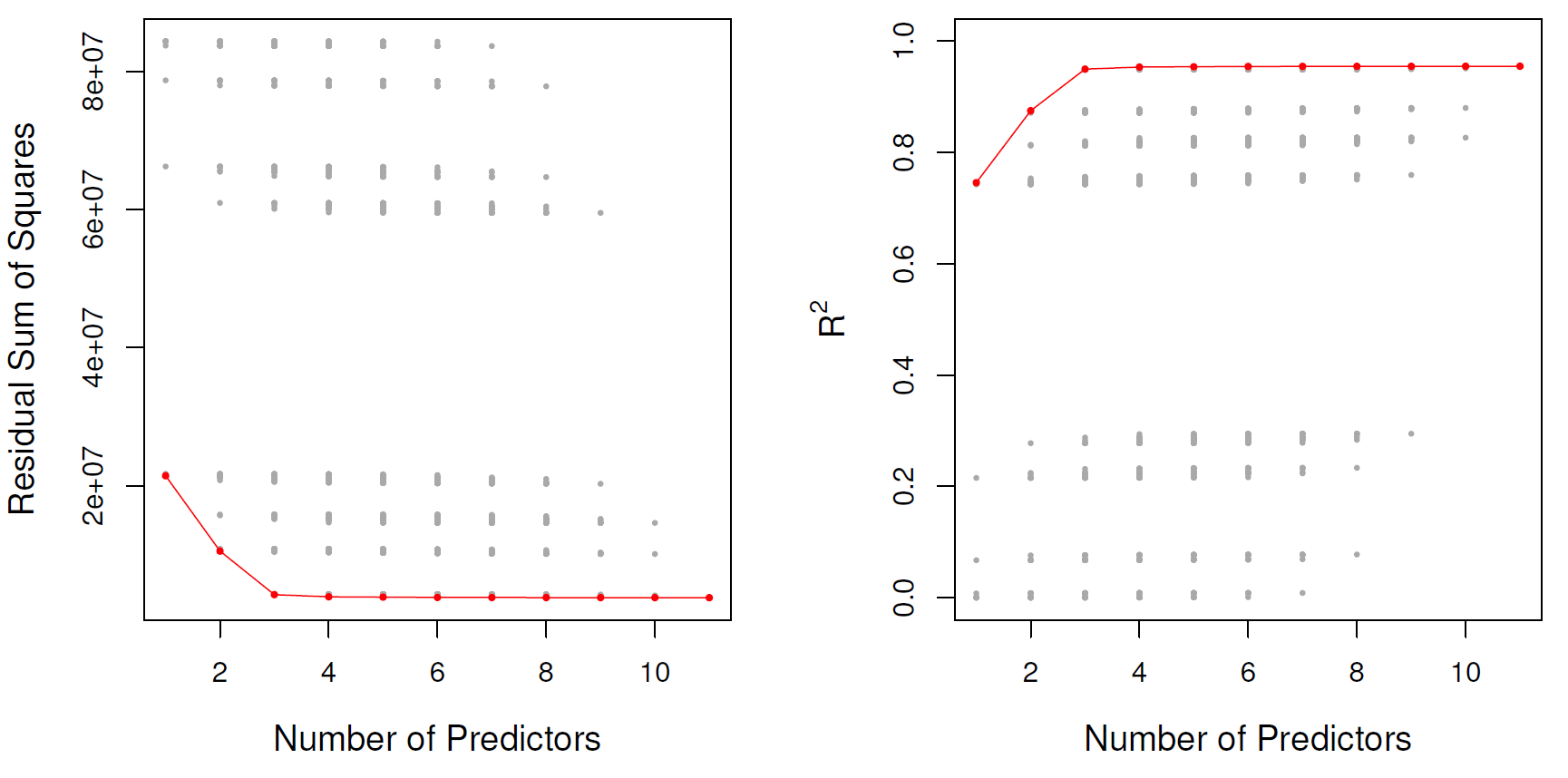
Credit data set.The Bayesian information criterion (BIC) is defined as \text{BIC} = d \ln(n) - 2 \ln(\hat{L}) where d and \hat{L} are defined as for the AIC. In the case of Linear Regression (strong assumptions) with d predictors, this is equivalent to \frac{1}{n}(\text{RSS}+\ln(n) \, d\hat{\sigma}^2) Note that \ln(n) > 2 for n > 7, so BIC gives a heavier penalty on adding predictors.
Adjusted R^2 with d predictors 1-\frac{\text{RSS}/(n-d-1)}{\text{TSS}/(n-1)} Again, the idea is to give a “penalty” for adding predictors to the model. This criteria is widely used, though its theoretical backing is not as strong as other measures.
Credit datasetBest subset selection algorithm:
Question for a Champion: in Step 2.b., why are we relying on R^2, if we argued before that it is flawed?
Algorithm:
(note that \mathcal{M}_p denotes the “full model”, i.e., with all p predictors included).
| # Variables | Best subset | Forward stepwise |
|---|---|---|
| 1 | rating | rating |
| 2 | rating, income | rating, income |
| 3 | rating, income, student | rating, income, student |
| 4 | cards, income, student, limit | rating, income, student, limit |
Recall the below data was generated by Y = 1 + 0.2 \times X^2 + \epsilon where X \sim U[0,10] and \epsilon \sim N(0, \sigma^2=0.01) with n = 500.
Mean of the residuals: -1.431303e-16 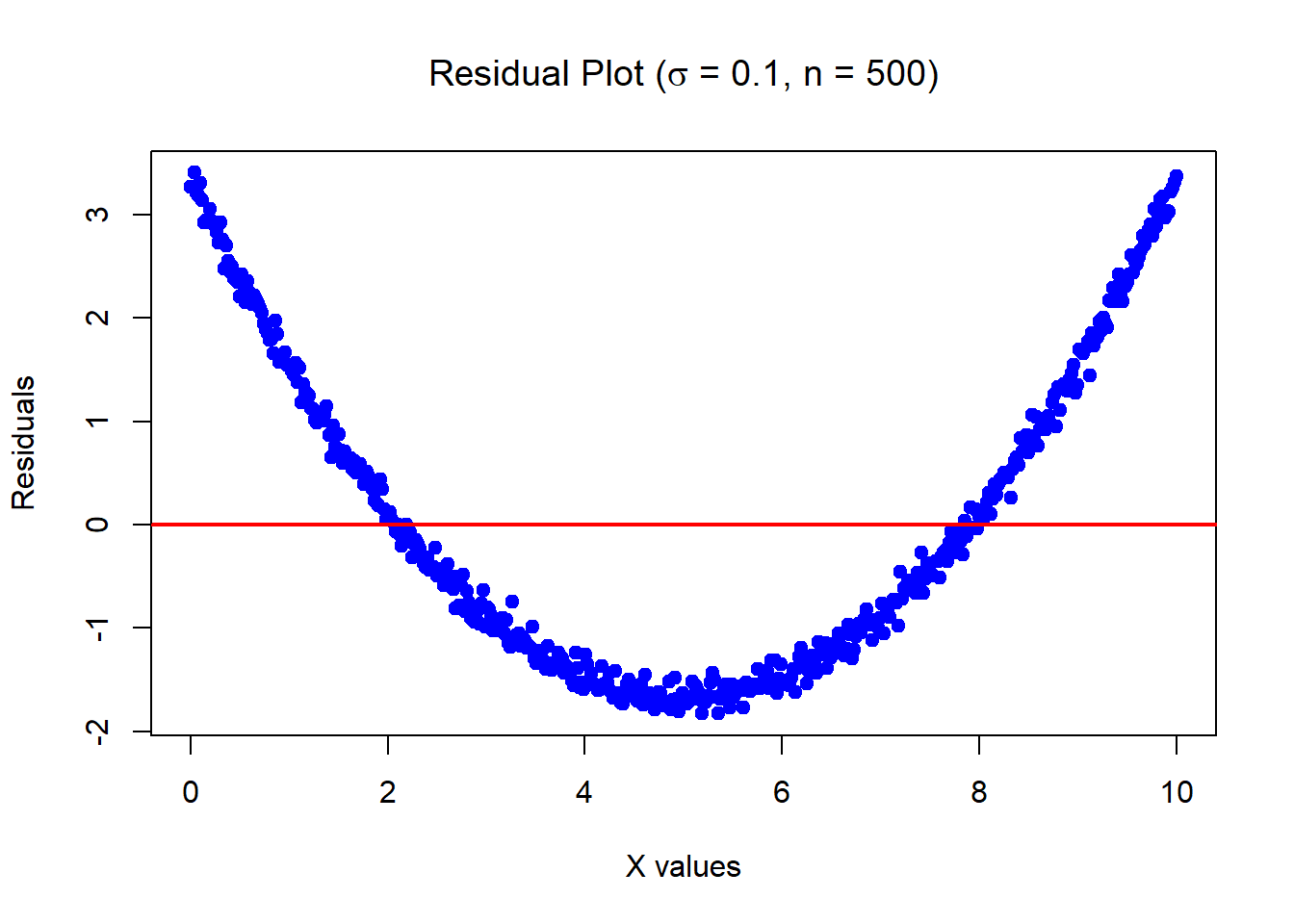
Example: residuals vs fitted for MPG vs Horsepower:
In this example, the quadratic model removes much of the pattern (more on this later).
The following are two regression outputs for Y (LHS) and \ln Y (RHS)
In this example, the log transformation removed much of the heteroscedasticity.
An outlier is a point for which the response “y_i” is far from the value predicted by the model (otherwise said, it has a large residual y_i - \hat{y}_i).
The below data was generated by Y = 1 - 0.5\times X + \epsilon where X \sim U[0,10] and \epsilon \sim N(0,1) with n = 30. We have added one high leverage point (made a red ‘+’ on the scatterplot).
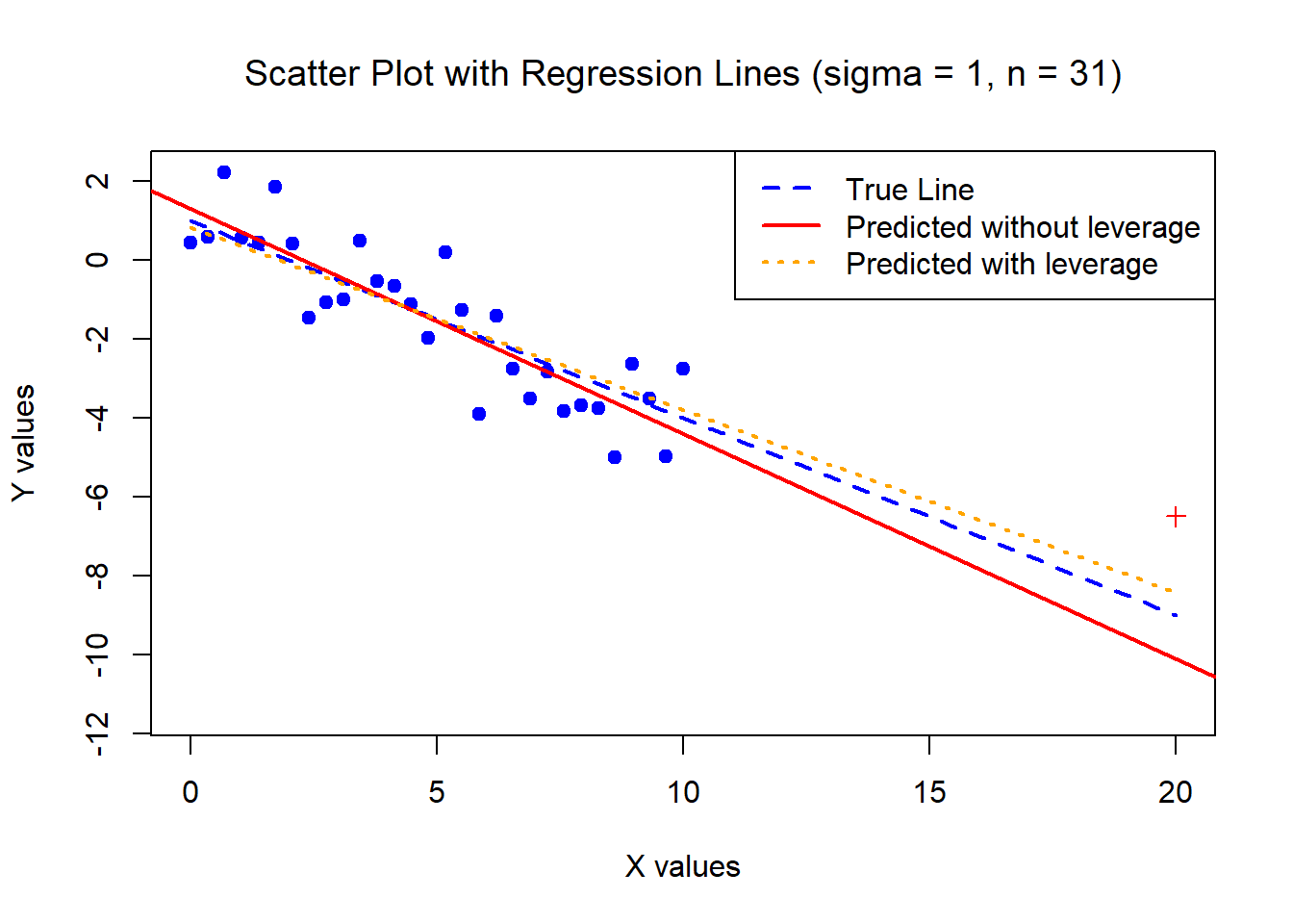
Credit dataset used.balance regressed onto age and limit. Predictors have low collinearity.balance regressed onto rating and limit. Predictors have high collinearity.The below data was generated by Y = 1 - 0.7\times X_1 + X_2 + \epsilon where \epsilon \sim N(0,1), X_1 \sim U[0,10], X_2 = 2X_1. Note n = 30.
The below data was generated by Y = 1 - 0.7\times X_1 + X_2 + \epsilon where \epsilon \sim N(0,1) and X_1 \sim U[0,10], X_2 = 2X_1 + \varepsilon, where \varepsilon \sim N(0,10^{-8}) is a small quantity (so the fitting “works”). Note n=30.
Call:
lm(formula = Y ~ X1 + X2)

Residuals:
     Min       1Q   Median       3Q      Max
-2.32126 -0.46578  0.02207  0.54006  1.89817

Coefficients:
              Estimate Std. Error t value Pr(>|t|)
(Intercept)  5.192e-01  3.600e-01   1.442   0.1607
X1           5.958e+04  3.268e+04   1.823   0.0793 .
X2          -2.979e+04  1.634e+04  -1.823   0.0793 .
---
Signif. codes:  0 '***' 0.001 '**' 0.01 '*' 0.05 '.' 0.1 ' ' 1

Residual standard error: 0.8538 on 27 degrees of freedom
Multiple R-squared:  0.9614,    Adjusted R-squared:  0.9585
F-statistic: 335.9 on 2 and 27 DF,  p-value: < 2.2e-16
Loading required package: carData
Attaching package: 'car'The following object is masked from 'package:dplyr':
recodeThe following object is masked from 'package:purrr':
someVIF for X1: 360619740351 VIF for X2: 360619740351 How to correctly use/don’t use confounding variables?
Many methods we will see in the rest of the course expand the scope of linear models:
Recall from ACTL2131/ACTL5101, we have the following sum of squares:
\begin{aligned} S_{xx} & =\sum_{i=1}^{n}(x_i-\overline{x})^2 &\implies s_x^2=\frac{S_{xx}}{n-1} \\ S_{yy} & =\sum_{i=1}^{n}(y_i-\overline{y})^2 &\implies s_y^2=\frac{S_{yy}}{n-1}\\ S_{xy} & =\sum_{i=1}^{n}(x_i-\overline{x})(y_i-\overline{y}) &\implies s_{xy}=\frac{S_{xy}}{n-1}, \end{aligned} Here s_x^2, s_y^2 (and s_{xy}) denote sample (co-)variance.
Rationale for \beta_1: Recall that \hat{\beta}_1 is unbiased and \text{Var}(\hat{\beta}_1)=\sigma^2/S_{xx}. However \sigma^2 is usually unknown, and estimated by s^2 so, under the strong assumptions, we have: \frac{\hat{\beta}_1-\beta_1 }{ s/ \sqrt{S_{xx}}} = \left.{\underset{\mathcal{N}(0,1)}{\underbrace{\frac{\hat{\beta}_1-\beta_1}{\sigma/ \sqrt{S_{xx}}}}}}\right/{\underset{\sqrt{\chi^2_{n-2}/(n-2)}}{\underbrace{\sqrt{\frac{\frac{(n-2)\cdot s^2}{\sigma^2}}{n-2}}}}} \sim t_{n-2} as \epsilon_i \overset{\text{i.i.d.}}{\sim} \mathcal{N}(0,\sigma^2) then \frac{(n-2)\cdot s^2}{\sigma^2} = \frac{\sum_{i=1}^{n}(y_i-\hat{\beta}_0-\hat{\beta}_1\cdot x_i)^2}{\sigma^2} \sim\chi^2_{{n}-2}.
Note: Why do we lose two degrees of freedom? Because we estimated two parameters!
Similar rationale for \beta_0.
Suppose x=x_{0} is a specified value of the out of sample regressor variable and we want to predict the corresponding Y value associated with it. The mean of Y is: \begin{aligned} \mathbb{E}[ Y \mid x_0 ] &= \mathbb{E}[ \beta_0 +\beta_1 x \mid x=x_0 ] \\ &= \beta_0 + \beta_1 x_0. \end{aligned}
Our (unbiased) estimator for this mean (also the fitted value of y_0) is: \hat{y}_{0}=\hat{\beta}_0+\hat{\beta}_1x_{0}. The variance of this estimator is: \text{Var}( \hat{y}_0 ) = \left( \frac{1}{n} + \frac{(\overline{x}-x_0)^2}{S_{xx}}\right) \sigma ^{2} = \text{SE}(\hat{y}_0)^2
Proof: See Lab questions.
Using the strong assumptions, the 100\left( 1-\alpha\right) \% confidence interval for \beta_0 +\beta_1 x_{0} (mean of Y) is: \underbrace{\bigl(\hat{\beta}_0 + \hat{\beta}_1 x_0 \bigr)}_{\hat{y}_0} \pm t_{1-\alpha/2,n-2}\times {\underbrace{s\sqrt{ \dfrac{1}{n}+\dfrac{\left(\overline{x}-x_{0}\right) ^{2}}{S_{xx}}}}_{\hat{\text{SE}}(\hat{y}_0)}} ,
as we have \hat{y}_{0} \sim \mathcal{N}( \beta_0 +\beta_1 x_{0}, \text{SE}(\hat{y}_0)^2 %={\left( \dfrac{1}{n}+\frac{\left( \overline{x}-x_{0}\right) ^{2}}{S_{xx}}\right)\sigma ^{2}} )
and \frac{\hat{y}_{0} - (\beta_0 +\beta_1 x_0)}{\hat{\text{SE}}(\hat{y}_0)} %=\frac{\hat{y}_{0} - \left( \beta_0 +\beta_1 x_{0}\right)}{s\sqrt{\dfrac{1}{n}+\dfrac{\left( \overline{x}-x_{0}\right)^{2}}{S_{xx}} }} \sim t(n-2).
Similar rationale to slide.
A prediction interval is a confidence interval for the actual value of a Y_i (not for its mean \beta_0 + \beta_1 x_i). We base our prediction of Y_i (given {X}=x_i) on: {\hat{y}}_i={\hat{\beta}}_0+{\hat{\beta}}_1x_i. The error in our prediction is: \begin{aligned} {Y}_i-{\hat{y}}_i=\beta_0+\beta_1x_i+{\epsilon}_i-{\hat{y}}_i=\mathbb{E}[{Y}|{X}=x_i]-{\hat{y}}_i+{\epsilon}_i. \end{aligned} with \mathbb{E}\left[{Y}_i-{\hat{y}}_i|{{X}}={x},{X}=x_i\right]=0 , \text{ and } \text{Var}({Y}_i-{\hat{y}}_i|{{X}}={x},{X}=x_i)=\sigma^2\bigl(1+{1\over n}+{(\overline{x} - x_i)^2\over S_{xx}}\bigr) .
Proof: See Lab questions.
A 100(1-\alpha)% prediction interval for {Y}_i, the value of {Y} at {X}=x_i, is given by:
\begin{aligned} %&& {{\hat{y}}_i}\pm t_{1-\alpha/2,n-2}s\sqrt{1+\displaystyle{1\over n}+{(\overline{x} - x_i)^2\over S_{xx}}}\rule{140pt}{0pt}\\ %\equiv && {\underbrace{\hat{\beta}_0+\hat{\beta}_1x_i}_{\hat{y}_i}} \pm t_{1-\alpha/2,n-2}\cdot s\cdot\sqrt{1+\displaystyle{1\over n}+{(\overline{x} - x_i)^2\over S_{xx}}}, \end{aligned} as ({Y}_i-{\hat{y}}_i|{\underline{X}}=\underline{x},{X}=x_i) \sim \mathcal{N}\Bigl(0, \sigma^2\bigl(1 + \frac1n + \frac{(\overline{x} - x_i)^2}{S_{xx}}\bigr)\Bigr) , \text{ and } \frac{Y_i- \hat{y}_i}{s\sqrt{1 + \frac1n + \frac{(\overline{x} - x_i)^2}{S_{xx}}}} \sim t_{n-2}.
Check this website on spurious correlations.↩︎