Show the package imports
library(tidyverse)
library(rpart)
library(rpart.plot)
library(glmnet)library(tidyverse)
library(rpart)
library(rpart.plot)
library(glmnet)James et al. (2021): Chapter 5 (skipping bootstrap sections), and Section 6.2 (skipping Bayesian interpretation).
Scenario: use head circumference (mm) to predict age (weeks) of a fetal baby
\boldsymbol{x} = \begin{pmatrix} 105 \\ 120 \\ 110 \\ 117 \\ \end{pmatrix}, \quad \boldsymbol{y} = \begin{pmatrix} 20 \\ 24 \\ 22 \\ 23 \\ \end{pmatrix}, \quad \hat{\boldsymbol{y}} = \begin{pmatrix} 20.3 \\ 24.0 \\ 21.5 \\ 23.2 \\ \end{pmatrix}
\hat{y}(x) = \beta_0 + \beta_1 x
circumference <- c(105, 120, 110, 117)
age <- c(20, 24, 22, 23)
model <- lm(age ~ circumference)
print(coef(model))
(Intercept) circumference
-5.5905797 0.2463768 predict(model, newdata = data.frame(circumference)) 1 2 3 4
20.27899 23.97464 21.51087 23.23551 \boldsymbol{y} = \begin{pmatrix} 20 \\ 24 \\ 22 \\ 23 \\ \end{pmatrix}, \quad \hat{\boldsymbol{y}} = \begin{pmatrix} 20.3 \\ 24.0 \\ 21.5 \\ 23.2 \\ \end{pmatrix}, \quad \boldsymbol{y} - \hat{\boldsymbol{y}} = \begin{pmatrix} -0.3 \\ 0 \\ 0.5 \\ -0.2 \\ \end{pmatrix}.
# Predictions
predicted_age <- predict(model, newdata = data.frame(circumference = circumference))

# Calculate ranges
x_range <- max(circumference) - min(circumference)
y_range <- max(age) - min(age)

# Calculate optimal aspect ratio
optimal_aspect_ratio <- x_range / y_range

# Create data frame for plotting
data <- data.frame(circumference, age, predicted_age)
data$error <- abs(data$age - data$predicted_age)

mse <- mean(data$error^2)

# Plotting
ggplot(data, aes(x = circumference, y = age)) +
  geom_point() +
  geom_line(aes(y = predicted_age)) +
  geom_segment(aes(xend = circumference, yend = predicted_age), linetype = 'dashed') +
  geom_rect(aes(xmin = circumference, xmax = circumference + error, ymin = pmin(age, predicted_age), ymax = pmin(age, predicted_age) + error),
            fill = 'red', alpha = 0.3) +
  xlab('Head Circumference (mm)') +
  ylab('Age (weeks)') +
  theme_minimal() +
  theme(aspect.ratio = 1 / optimal_aspect_ratio) +
  theme(legend.position = 'none') +
  ggtitle(paste('MSE = ', round(mse, 2)))
\text{MSE} = \frac{1}{n} \sum_{i=1}^n (y_i - \hat{y}_i)^2 = \frac{1}{4} \Bigl[ (-0.3)^2 + 0^2 + 0.5^2 + (-0.2)^2 \Bigr] = 0.09.
\text{If we instead had } \boldsymbol{y} = \begin{pmatrix} \textcolor{red}{10} & 24 & 22 & 23 \end{pmatrix}^\top.
circumference <- c(105, 120, 110, 117)
age <- c(10, 24, 22, 23)
new_model <- lm(age ~ circumference)

# Predictions
predicted_age <- predict(model, newdata = data.frame(circumference = circumference))

# Calculate ranges
x_range <- max(circumference) - min(circumference)
y_range <- max(age) - min(age)

# Calculate optimal aspect ratio
optimal_aspect_ratio <- x_range / y_range

# Create data frame for plotting
data <- data.frame(circumference, age, predicted_age)
data$error <- abs(data$age - data$predicted_age)

mse <- mean(data$error^2)

# Plotting
ggplot(data, aes(x = circumference, y = age)) +
  geom_point() +
  geom_line(aes(y = predicted_age)) +
  geom_segment(aes(xend = circumference, yend = predicted_age), linetype = 'dashed') +
  geom_rect(aes(xmin = circumference, xmax = circumference + error, ymin = pmin(age, predicted_age), ymax = pmin(age, predicted_age) + error),
            fill = 'red', alpha = 0.3) +
  xlab('Head Circumference (mm)') +
  ylab('Age (weeks)') +
  theme_minimal() +
  theme(aspect.ratio = 1 / optimal_aspect_ratio) +
  theme(legend.position = 'none') +
  ggtitle(paste('MSE = ', round(mse, 2)))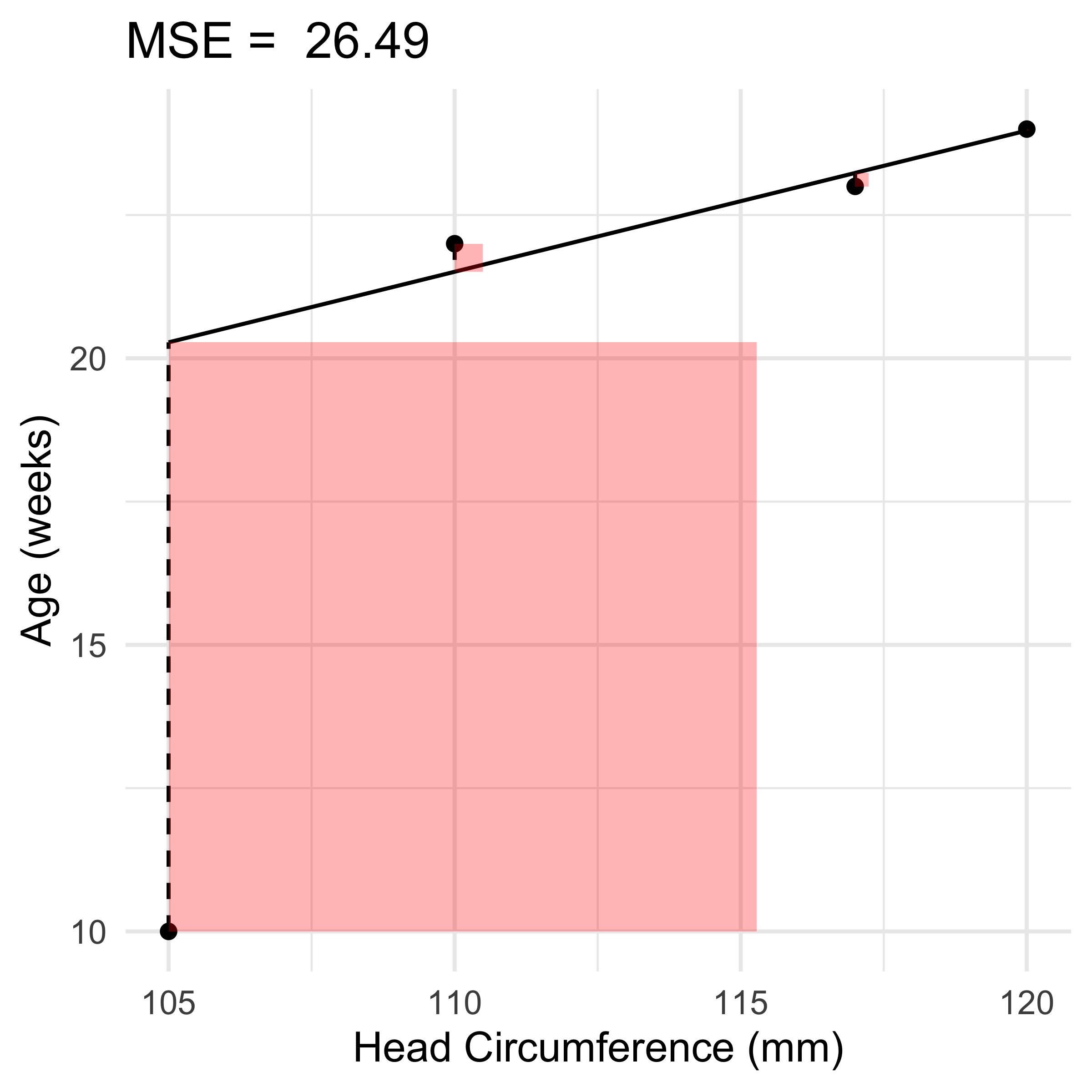
new_model <- lm(age ~ circumference)

# Predictions
predicted_age <- predict(new_model, newdata = data.frame(circumference = circumference))

# Calculate ranges
x_range <- max(circumference) - min(circumference)
y_range <- max(age) - min(age)

# Calculate optimal aspect ratio
optimal_aspect_ratio <- x_range / y_range

# Create data frame for plotting
data <- data.frame(circumference, age, predicted_age)
data$error <- abs(data$age - data$predicted_age)

mse <- mean(data$error^2)

# Plotting
ggplot(data, aes(x = circumference, y = age)) +
  geom_point() +
  geom_line(aes(y = predicted_age)) +
  geom_segment(aes(xend = circumference, yend = predicted_age), linetype = 'dashed') +
  geom_rect(aes(xmin = circumference, xmax = circumference + error, ymin = pmin(age, predicted_age), ymax = pmin(age, predicted_age) + error),
            fill = 'red', alpha = 0.3) +
  xlab('Head Circumference (mm)') +
  ylab('Age (weeks)') +
  theme_minimal() +
  theme(aspect.ratio = 1 / optimal_aspect_ratio) +
  theme(legend.position = 'none') +
  ggtitle(paste('MSE = ', round(mse, 2)))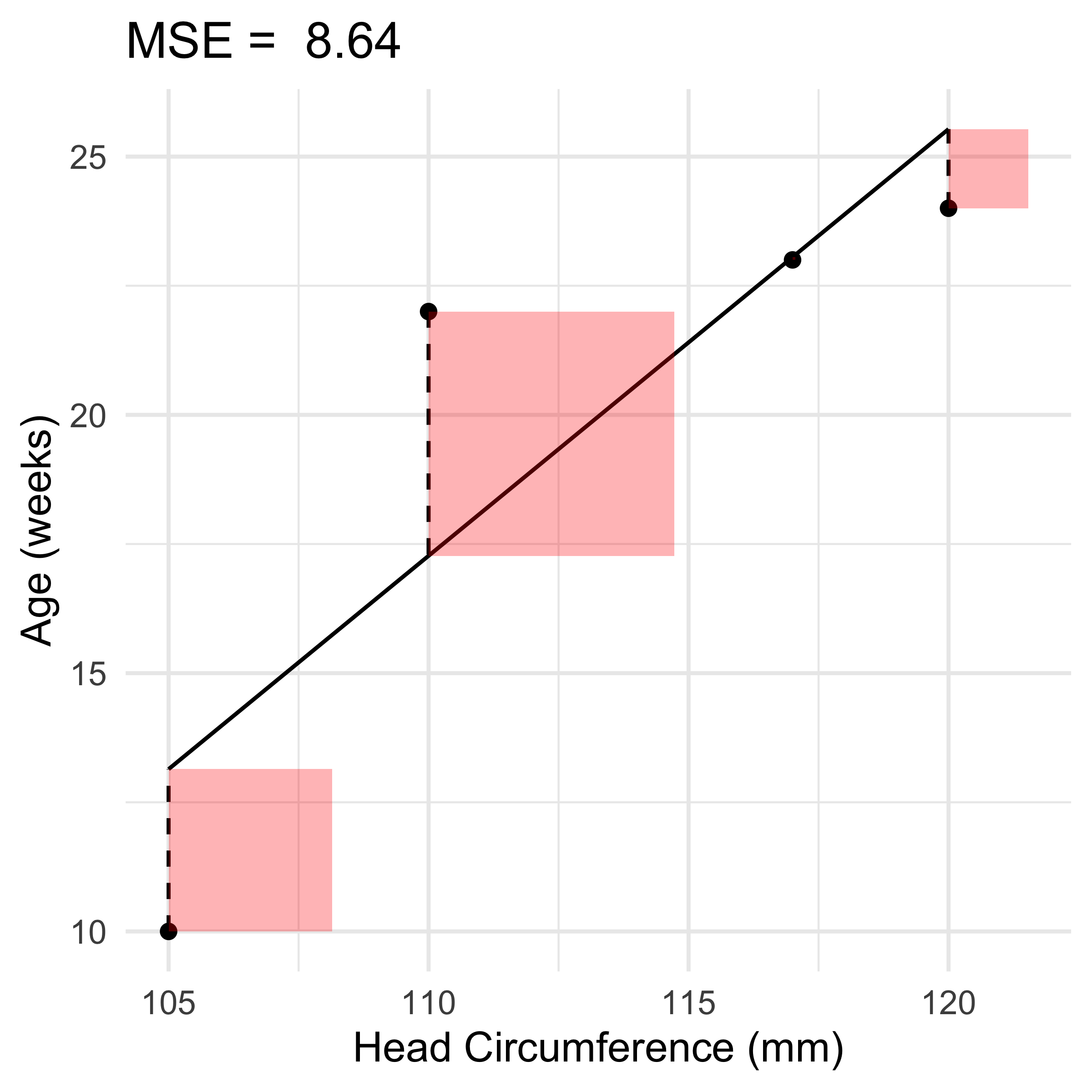
Scenario: use temperature (^\circ C) and humidity (%) to predict rainfall (mm)
\boldsymbol{X} = \begin{pmatrix} 27 & 80 \\ 32 & 70 \\ 28 & 72 \\ 22 & 86 \\ \end{pmatrix}, \quad \boldsymbol{y} = \begin{pmatrix} 6 \\ 7 \\ 6 \\ 4 \\ \end{pmatrix}, \quad \hat{\boldsymbol{y}} = \begin{pmatrix} 5.7 \\ 7.2 \\ 5.9 \\ 4.2 \\ \end{pmatrix}
\hat{y}(\boldsymbol{x}) = \beta_0 + \beta_1 x_1 + \beta_2 x_2 + \dots + \beta_p x_p = \beta_0 + \left \langle \boldsymbol{\beta}, \boldsymbol{x} \right \rangle
weather <- data.frame(temperature = c(27, 32, 28, 22), humidity = c(80, 70, 72, 86))
rainfall <- c(6, 7, 6, 4)
model <- lm(rainfall ~ temperature + humidity, data = weather)
summary(model)$coefficients
Estimate Std. Error t value Pr(>|t|)
(Intercept) -5.51001821 10.45422801 -0.5270612 0.6912003
temperature 0.34244080 0.15162225 2.2585129 0.2653588
humidity 0.02504554 0.08434494 0.2969418 0.8162405predict(model, newdata = weather) 1 2 3 4
5.739526 7.201275 5.881603 4.177596 Scenario: use temperature (^\circ C) and humidity (%) to predict rainfall (mm)
\boldsymbol{X} = \begin{pmatrix} \textcolor{grey}{1} & 27 & 80 \\ \textcolor{grey}{1} & 32 & 70 \\ \textcolor{grey}{1} & 28 & 72 \\ \textcolor{grey}{1} & 22 & 86 \\ \end{pmatrix}, \quad \boldsymbol{y} = \begin{pmatrix} 6 \\ 7 \\ 6 \\ 4 \\ \end{pmatrix}, \quad \hat{\boldsymbol{y}} = \begin{pmatrix} 5.7 \\ 7.2 \\ 5.9 \\ 4.2 \\ \end{pmatrix}
\hat{y}(\boldsymbol{x}) = \beta_0 x_0 + \beta_1 x_1 + \beta_2 x_2 + \dots + \beta_p x_p = \langle \boldsymbol{\beta}, \boldsymbol{x} \rangle
as.matrix(weather) temperature humidity
[1,] 27 80
[2,] 32 70
[3,] 28 72
[4,] 22 86X <- model.matrix(rainfall ~ temperature + humidity, data = weather)
X (Intercept) temperature humidity
1 1 27 80
2 1 32 70
3 1 28 72
4 1 22 86
attr(,"assign")
[1] 0 1 2\boldsymbol{\beta} = (\boldsymbol{X}^\top\boldsymbol{X})^{-1} \boldsymbol{X}^\top \boldsymbol{y}
model <- lm(rainfall ~ temperature +
        humidity, data = weather)
coef(model)
(Intercept) temperature humidity
-5.51001821 0.34244080 0.02504554 y <- rainfall
beta <- solve(t(X) %*% X) %*% t(X) %*% y
beta [,1]
(Intercept) -5.51001821
temperature 0.34244080
humidity 0.02504554\hat{\boldsymbol{y}} = \boldsymbol{X} \boldsymbol{\beta}.
predict(model, newdata = weather) 1 2 3 4
5.739526 7.201275 5.881603 4.177596 X %*% beta [,1]
1 5.739526
2 7.201275
3 5.881603
4 4.177596Scenario: use temperature (z-score) and humidity (z-score) to predict rainfall (mm) \boldsymbol{X} = \begin{pmatrix} \textcolor{grey}{1} & -0.06 & 0.41 \\ \textcolor{grey}{1} & 1.15 & -0.95 \\ \textcolor{grey}{1} & 0.18 & -0.68 \\ \textcolor{grey}{1} & -1.28 & 1.22 \\ \end{pmatrix}, \quad \boldsymbol{y} = \begin{pmatrix} 6 \\ 7 \\ 6 \\ 4 \\ \end{pmatrix}, \quad \hat{\boldsymbol{y}} = \begin{pmatrix} 5.7 \\ 7.2 \\ 5.9 \\ 4.2 \\ \end{pmatrix}
\hat{y}(\boldsymbol{x}) = \beta_0 x_0 + \beta_1 x_1 + \beta_2 x_2 + \dots + \beta_p x_p = \langle \boldsymbol{\beta}, \boldsymbol{x} \rangle
weather <- data.frame(temperature = c(27, 32, 28, 22), humidity = c(80, 70, 72, 86))
weather <- data.frame(scale(weather))
rainfall <- c(6, 7, 6, 4)
model <- lm(rainfall ~ temperature + humidity, data = weather)
summary(model)$coefficients
Estimate Std. Error t value Pr(>|t|)
(Intercept) 5.750000 0.1961608 29.3126889 0.02170981
temperature 1.408455 0.6236204 2.2585129 0.26535876
humidity 0.185179 0.6236204 0.2969418 0.81624051predict(model, newdata = weather) 1 2 3 4
5.739526 7.201275 5.881603 4.177596 Scenario: use property type to predict its sale price ($)
\boldsymbol{x} = \begin{pmatrix} \textcolor{red}{\text{Unit}} \\ \textcolor{green}{\text{TownHouse}} \\ \textcolor{green}{\text{TownHouse}} \\ \textcolor{blue}{\text{House}} \\ \end{pmatrix} \longrightarrow \boldsymbol{X} = \begin{pmatrix} \textcolor{grey}{1} & 1 & 0 \\ \textcolor{grey}{1} & 0 & 1 \\ \textcolor{grey}{1} & 0 & 1 \\ \textcolor{grey}{1} & 0 & 0 \\ \end{pmatrix}, \quad \boldsymbol{y} = \begin{pmatrix} 300000 \\ 500000 \\ 510000 \\ 700000 \\ \end{pmatrix}, \quad \hat{\boldsymbol{y}} = \begin{pmatrix} 300000 \\ 505000 \\ 505000 \\ 700000 \\ \end{pmatrix}
\hat{y}(x) = \beta_0 + \beta_1 \underbrace{I(x = \textcolor{red}{\text{Unit}})}_{=: x_1} + \beta_2 \underbrace{I(x = \textcolor{green}{\text{TownHouse}})}_{=: x_2} = \beta_0 + \beta_1 x_1 + \beta_2 x_2
type <- factor(c("Unit", "TownHouse", "TownHouse", "House"))
price <- c(300000, 500000, 510000, 700000)
model <- lm(price ~ type)
summary(model)$coefficients
Estimate Std. Error t value Pr(>|t|)
(Intercept) 700000 7071.068 98.99495 0.006430612
typeTownHouse -195000 8660.254 -22.51666 0.028254710
typeUnit -400000 10000.000 -40.00000 0.015912180predict(model, newdata = data.frame(type)) 1 2 3 4
300000 505000 505000 700000 Scenario: use property type to predict its sale price ($)
\boldsymbol{x} = \begin{pmatrix} \textcolor{red}{\text{Unit}} \\ \textcolor{green}{\text{TownHouse}} \\ \textcolor{green}{\text{TownHouse}} \\ \textcolor{blue}{\text{House}} \\ \end{pmatrix} \longrightarrow \boldsymbol{X} = \begin{pmatrix} \textcolor{grey}{1} & 0 & 0 \\ \textcolor{grey}{1} & 1 & 0 \\ \textcolor{grey}{1} & 1 & 0 \\ \textcolor{grey}{1} & 0 & 1 \\ \end{pmatrix}, \quad \boldsymbol{y} = \begin{pmatrix} 300000 \\ 500000 \\ 510000 \\ 700000 \\ \end{pmatrix}, \quad \hat{\boldsymbol{y}} = \begin{pmatrix} 300000 \\ 505000 \\ 505000 \\ 700000 \\ \end{pmatrix}
\hat{y}(x) = \beta_0 + \beta_1 \underbrace{I(x = \textcolor{green}{\text{TownHouse}})}_{=: x_1} + \beta_2 \underbrace{I(x = \textcolor{blue}{\text{House}})}_{=: x_2} = \beta_0 + \beta_1 x_1 + \beta_2 x_2
type <- factor(c("Unit", "TownHouse", "TownHouse", "House"), levels = c("Unit", "TownHouse", "House"))
price <- c(300000, 500000, 510000, 700000)
model <- lm(price ~ type)
summary(model)$coefficients
Estimate Std. Error t value Pr(>|t|)
(Intercept) 300000 7071.068 42.42641 0.01500249
typeTownHouse 205000 8660.254 23.67136 0.02687811
typeHouse 400000 10000.000 40.00000 0.01591218predict(model, newdata = data.frame(type)) 1 2 3 4
300000 505000 505000 700000 Scenario: use property type to predict its sale price ($000,000’s)
\boldsymbol{x} = \begin{pmatrix} \textcolor{red}{\text{Unit}} \\ \textcolor{green}{\text{TownHouse}} \\ \textcolor{green}{\text{TownHouse}} \\ \textcolor{blue}{\text{House}} \\ \end{pmatrix} \longrightarrow \boldsymbol{X} = \begin{pmatrix} \textcolor{grey}{1} & 0 & 0 \\ \textcolor{grey}{1} & 1 & 0 \\ \textcolor{grey}{1} & 1 & 0 \\ \textcolor{grey}{1} & 0 & 1 \\ \end{pmatrix}, \quad \boldsymbol{y} = \begin{pmatrix} 0.3 \\ 0.5 \\ 0.51 \\ 0.7 \\ \end{pmatrix}, \quad \hat{\boldsymbol{y}} = \begin{pmatrix} 0.3 \\ 0.505 \\ 0.505 \\ 0.7 \\ \end{pmatrix}
\hat{y}(x) = \beta_0 + \beta_1 \underbrace{I(x = \textcolor{green}{\text{TownHouse}})}_{=: x_1} + \beta_2 \underbrace{I(x = \textcolor{blue}{\text{House}})}_{=: x_2} = \beta_0 + \beta_1 x_1 + \beta_2 x_2
type <- factor(c("Unit", "TownHouse", "TownHouse", "House"), levels = c("Unit", "TownHouse", "House"))
price <- c(0.3, 0.5, 0.51, 0.7)
model <- lm(price ~ type)
summary(model)$coefficients
Estimate Std. Error t value Pr(>|t|)
(Intercept) 0.300 0.007071068 42.42641 0.01500249
typeTownHouse 0.205 0.008660254 23.67136 0.02687811
typeHouse 0.400 0.010000000 40.00000 0.01591218predict(model, newdata = data.frame(type)) 1 2 3 4
0.300 0.505 0.505 0.700 Imagine you had dataset with 157,209 rows and one covariate column was ‘date of birth’. There were 27,485 unique values for the date of birth column. You make a linear regression with the date of birth as an input, and treat it as a categorical variable (the default behaviour for text data in R).
R would make a design matrix of size 157,209 \times 27,485. This has 4,320,889,365 numbers in it. Each number is stored as 8 bytes, so the matrix is roughly 34,000,000,000 \text{ bytes} = 34,000,000 \text{ KB} = 34,000 \text{ MB} = 34 \text{ GB}.
Question: How do we avoid this situation of crashing our computer with an ‘out of memory’ error?
Solution: Don’t train on the date of birth — at least, not as a categorical variable. Turn it into a numerical variable, e.g. age. If the date column were not ‘date of birth’, maybe calculate the number of days since some reference date, or split into day, month, year columns.
Scenario: use tumour radius (mm) and ages (years) to predict benign or malignant \boldsymbol{X} = \begin{pmatrix} \textcolor{grey}{1} & 14.8 & 48 \\ \textcolor{grey}{1} & 16.4 & 49 \\ \textcolor{grey}{1} & 15.5 & 47 \\ \textcolor{grey}{1} & 14.2 & 46 \\ \end{pmatrix}, \quad \boldsymbol{y} = \begin{pmatrix} \text{Benign} \\ \text{Malignant} \\ \text{Benign} \\ \text{Malignant} \\ \end{pmatrix}, \quad \hat{\boldsymbol{y}} = \begin{pmatrix} ? \\ ? \\ ? \\ ? \\ \end{pmatrix}
Step 1: Make a linear prediction \beta_0 + \beta_1 x_1 + \dots + \beta_p x_p , \quad \text{a.k.a.} \quad \langle \boldsymbol{\beta}, \boldsymbol{x} \rangle.
Step 2: Shove it through some function to make it a probability \sigma(\langle \boldsymbol{\beta}, \boldsymbol{x} \rangle) Interpret that as being the probability of the positive class.
Step 3: Make a decision based on that probability. E.g., if the probability is greater than 0.5, predict the positive class.
Scenario: use tumour radius (mm) and ages (years) to predict benign or malignant \boldsymbol{X} = \begin{pmatrix} \textcolor{grey}{1} & 14.8 & 48 \\ \textcolor{grey}{1} & 16.4 & 49 \\ \textcolor{grey}{1} & 15.5 & 47 \\ \textcolor{grey}{1} & 14.2 & 46 \\ \end{pmatrix}, \quad \boldsymbol{y} = \begin{pmatrix} \text{Benign} \\ \textbf{\text{Malignant}} \\ \text{Benign} \\ \textbf{\text{Malignant}} \\ \end{pmatrix}, \quad \boldsymbol{X} \boldsymbol{\beta} = \begin{pmatrix} -0.46 \\ 0.18 \\ 0.37 \\ -0.09 \\ \end{pmatrix}
df <- data.frame(radius = c(14.8, 16.4, 15.5, 14.2), age = c(48, 49, 47, 46))
tumour <- factor(c("Benign", "Malignant", "Benign", "Malignant"))
model <- glm(tumour ~ radius + age, data = df, family = binomial)
Step 1: Make a linear prediction
linear <- predict(model, newdata = df, type = "link")
linear
1 2 3 4
-0.46393923 0.18380161 0.36575186 -0.08928047 X <- model.matrix(~ radius + age, data = df)
beta <- coef(model)
t(X %*% beta) 1 2 3 4
[1,] -0.4639392 0.1838016 0.3657519 -0.08928047# Plot the sigmoid function
sigmoid <- function(x) 1 / (1 + exp(-x))
x <- seq(-6, 6, 0.1)
y <- sigmoid(x)
df <- data.frame(x = x, y = y)
ggplot(df, aes(x = x, y = y)) +
geom_line(linewidth = 1.5) + # Thicker lines
xlab("x") +
ylab("y") +
ggtitle("Sigmoid function") +
theme(aspect.ratio = 1) # Square aspect ratio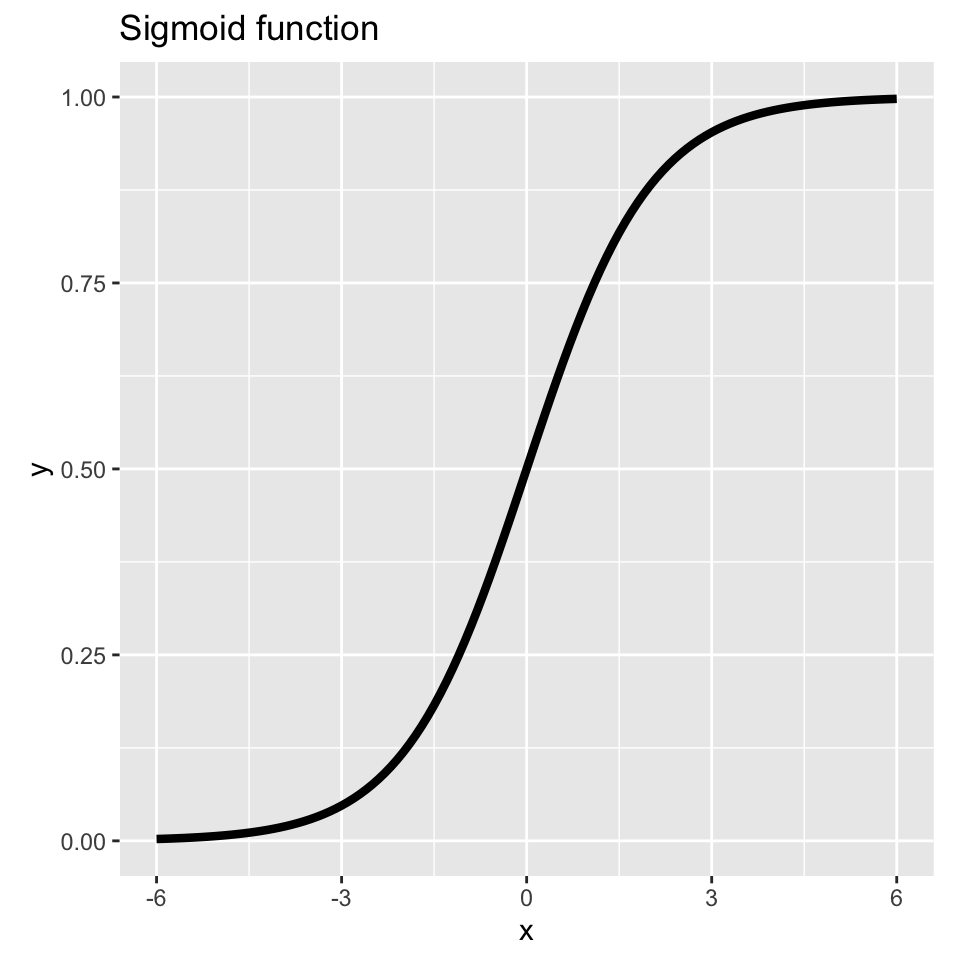
This give you logistic regression.
# Plot the Normal CDF function
x <- seq(-6, 6, 0.1)
y <- pnorm(x)
df <- data.frame(x = x, y = y)

ggplot(df, aes(x = x, y = y)) +
  geom_line(linewidth = 1.5) +  # Thicker lines
  xlab("x") +
  ylab("y") +
  ggtitle("Normal CDF function") +
  theme(aspect.ratio = 1)  # Square aspect ratio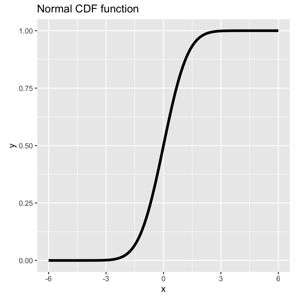
This gives you probit regression.
Scenario: use tumour radius (mm) and ages (years) to predict benign or malignant \boldsymbol{y} = \begin{pmatrix} \text{Benign} \\ \textbf{\text{Malignant}} \\ \text{Benign} \\ \textbf{\text{Malignant}} \\ \end{pmatrix}, \quad \boldsymbol{X} \boldsymbol{\beta} = \begin{pmatrix} -0.46 \\ 0.18 \\ 0.37 \\ -0.09 \\ \end{pmatrix}, \quad \sigma( \boldsymbol{X} \boldsymbol{\beta} ) = \begin{pmatrix} 39\% \\ 55\% \\ 59\% \\ 48\% \\ \end{pmatrix}
df <- data.frame(radius = c(14.8, 16.4, 15.5, 14.2), age = c(48, 49, 47, 46))
tumour <- factor(c("Benign", "Malignant", "Benign", "Malignant"))
model <- glm(tumour ~ radius + age, data = df, family = binomial)
Step 2: Shove it through some function to make it a probability
sigmoid <- function(x) 1 / (1 + exp(-x))
sigmoid(linear)
1 2 3 4
0.3860517 0.5458215 0.5904321 0.4776947 predict(model, newdata = df, type = "response") 1 2 3 4
0.3860517 0.5458215 0.5904321 0.4776947 Scenario: use tumour radius (mm) and ages (years) to predict benign or malignant \boldsymbol{y} = \begin{pmatrix} \text{Benign} \\ \textbf{\text{Malignant}} \\ \text{Benign} \\ \textbf{\text{Malignant}} \\ \end{pmatrix}, \quad \sigma( \boldsymbol{X} \boldsymbol{\beta} ) = \begin{pmatrix} 39\% \\ 55\% \\ 59\% \\ 48\% \\ \end{pmatrix} , \quad \hat{\boldsymbol{y}} = \begin{pmatrix} \text{Benign} \\ \text{Malignant} \\ \text{Malignant} \\ \text{Benign} \\ \end{pmatrix}
df <- data.frame(radius = c(14.8, 16.4, 15.5, 14.2), age = c(48, 49, 47, 46))
tumour <- factor(c("Benign", "Malignant", "Benign", "Malignant"))
model <- glm(tumour ~ radius + age, data = df, family = binomial)
predict_probs <- predict(model, newdata = df, type = "response")
round(100 * predict_probs, 2) 1 2 3 4
38.61 54.58 59.04 47.77 cutoff <- 0.5
predicted_tumours <- ifelse(predict_probs > cutoff, "Malignant", "Benign")
print(predicted_tumours) 1 2 3 4
"Benign" "Malignant" "Malignant" "Benign" Scenario: use tumour radius (mm) and ages (years) to predict benign or malignant \boldsymbol{y} = \begin{pmatrix} \textcolor{Green}{\text{Benign}} \\ \textcolor{Green}{\text{Malignant}} \\ \textcolor{Red}{\text{Benign}} \\ \textcolor{Red}{\text{Malignant}} \\ \end{pmatrix}, \quad \hat{\boldsymbol{y}} = \begin{pmatrix} \textcolor{Green}{\text{Benign}} \\ \textcolor{Green}{\text{Malignant}} \\ \textcolor{Red}{\text{Malignant}} \\ \textcolor{Red}{\text{Benign}} \\ \end{pmatrix}
Accuracy: \frac{1}{n}\sum_{i=1}^n I(y_i = \hat{y}_i)
Error rate: \frac{1}{n}\sum_{i=1}^n I(y_i \neq \hat{y}_i)
The word “accuracy” is used often used loosely when discussing models, particularly regression models. In the context of classification it has this specific meaning.
Scenario: use population density to predict the daily count of gun violence incidents
\boldsymbol{X} = \begin{pmatrix} \textcolor{grey}{1} & 10 \\ \textcolor{grey}{1} & 15 \\ \textcolor{grey}{1} & 12 \\ \textcolor{grey}{1} & 18 \\ \end{pmatrix}, \quad \boldsymbol{y} = \begin{pmatrix} 155 \\ 208 \\ 116 \\ 301 \\ \end{pmatrix}, \quad \hat{\boldsymbol{y}} = \begin{pmatrix} ? \\ ? \\ ? \\ ? \\ \end{pmatrix}
Step 1: Make a linear prediction \beta_0 + \beta_1 x_1 + \dots + \beta_p x_p , \quad \text{a.k.a.} \quad \langle \boldsymbol{\beta}, \boldsymbol{x} \rangle.
Step 2: Shove it through some function to make it positive \exp(\langle \boldsymbol{\beta}, \boldsymbol{x} \rangle) Interpret that as being the expected count.
Scenario: use population density to predict the daily count of gun violence incidents
\boldsymbol{X} = \begin{pmatrix} \textcolor{grey}{1} & 10 \\ \textcolor{grey}{1} & 15 \\ \textcolor{grey}{1} & 12 \\ \textcolor{grey}{1} & 18 \\ \end{pmatrix}, \quad \boldsymbol{y} = \begin{pmatrix} 155 \\ 208 \\ 116 \\ 301 \\ \end{pmatrix}, \quad \boldsymbol{X} \boldsymbol{\beta} = \begin{pmatrix} 4.82 \\ 5.35 \\ 5.03 \\ 5.67 \\ \end{pmatrix}, \quad \hat{\boldsymbol{\mu}} = \begin{pmatrix} 125.1 \\ 211.3 \\ 154.3 \\ 289.4 \\ \end{pmatrix}
guns <- data.frame(density = c(10, 15, 12, 18))
incidents <- c(155, 208, 116, 301)
model <- glm(incidents ~ density, data = guns, family = poisson)
summary(model)$coefficients
Estimate Std. Error z value Pr(>|z|)
(Intercept) 3.7803729 0.17881503 21.141248 3.321765e-99
density 0.1048546 0.01190339 8.808802 1.264908e-18predict(model, newdata = guns, type = "link") 1 2 3 4
4.828919 5.353192 5.038628 5.667756 predict(model, newdata = guns, type = "response") 1 2 3 4
125.0757 211.2817 154.2583 289.3844 model <- rpart(tumour ~ radius + age, data = df, control = rpart.control(minsplit = 2))
rpart.plot(model)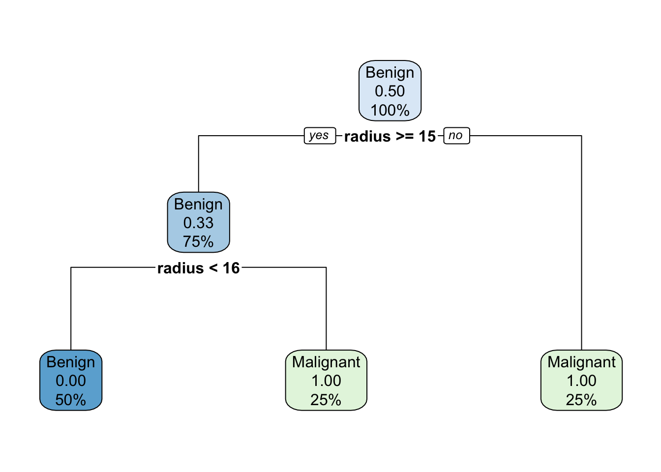
“This large dataset contains job descriptions and rankings among various criteria such as work-life balance, income, culture, etc. The data covers the various industries in the UK. Great dataset for multidimensional sentiment analysis.”
Original dataset is 300 MB, so I just took a subset of it. Focused on firms that have the word “University” in their name.

Rankings are 1–5:
overall_rating: rating for the job (target)work_life_balance: sub-rating: work-life balanceculture_values: sub-rating: culturediversity_inclusion: sub-rating: diversity and inclusioncareer_opp: sub-rating: career opportunitiescomp_benefits: sub-rating: compensation and benefitssenior_mgmt: sub-rating: senior managementLast two are coded: v - Positive, r - Mild, x - Negative, o - No opinion
recommend: recommend the firmceo_approv: approves firm’s CEOAvailable at https://laub.au/ml/data/uni_reviews.csv.
df_uni <- read.csv("uni_reviews.csv")
df_uni
# A tibble: 18,358 × 18
firm date_review job_title current location overall_rating work_life_balance
<chr> <chr> <chr> <chr> <chr> <int> <dbl>
1 Birm… 2012-06-28 " Operat… Curren… "Birmin… 5 4
2 Birm… 2014-04-23 " Inform… Curren… "Birmin… 4 5
3 Birm… 2014-05-05 " " Curren… "" 4 3
4 Birm… 2014-07-18 " Out Re… Curren… "Birmin… 2 5
5 Birm… 2014-12-05 " Profes… Curren… "Birmin… 5 5
6 Birm… 2015-07-28 " Anonym… Curren… "" 3 2
7 Birm… 2015-08-20 " Anonym… Former… "" 4 5
8 Birm… 2015-11-05 " Studen… Curren… "Birmin… 5 5
9 Birm… 2015-11-19 " Senior… Curren… "" 3 3
10 Birm… 2016-01-04 " Operat… Former… "Birmin… 4 5
# ℹ 18,348 more rows
# ℹ 11 more variables: culture_values <dbl>, diversity_inclusion <dbl>,
# career_opp <dbl>, comp_benefits <dbl>, senior_mgmt <dbl>, recommend <chr>,
# ceo_approv <chr>, outlook <chr>, headline <chr>, pros <chr>, cons <chr>summary(df_uni) firm date_review job_title current
Length:18358 Length:18358 Length:18358 Length:18358
Class :character Class :character Class :character Class :character
Mode :character Mode :character Mode :character Mode :character
location overall_rating work_life_balance culture_values
Length:18358 Min. :1.000 Min. :1.00 Min. :1.000
Class :character 1st Qu.:4.000 1st Qu.:3.00 1st Qu.:3.000
Mode :character Median :4.000 Median :4.00 Median :4.000
Mean :4.136 Mean :3.89 Mean :3.962
3rd Qu.:5.000 3rd Qu.:5.00 3rd Qu.:5.000
Max. :5.000 Max. :5.00 Max. :5.000
NA's :5316 NA's :5782
diversity_inclusion career_opp comp_benefits senior_mgmt
Min. :1.000 Min. :1.000 Min. :1.000 Min. :1.000
1st Qu.:4.000 1st Qu.:3.000 1st Qu.:3.000 1st Qu.:3.000
Median :5.000 Median :4.000 Median :4.000 Median :4.000
Mean :4.146 Mean :3.649 Mean :3.542 Mean :3.484
3rd Qu.:5.000 3rd Qu.:5.000 3rd Qu.:5.000 3rd Qu.:5.000
Max. :5.000 Max. :5.000 Max. :5.000 Max. :5.000
NA's :15448 NA's :5226 NA's :5452 NA's :5641
recommend ceo_approv outlook headline
Length:18358 Length:18358 Length:18358 Length:18358
Class :character Class :character Class :character Class :character
Mode :character Mode :character Mode :character Mode :character
pros cons
Length:18358 Length:18358
Class :character Class :character
Mode :character Mode :character
table(df_uni$firm) %>% sort(decreasing = TRUE) %>% head(10)
   University-of-Michigan University-College-London         Oxford-University
                     4185                      1259                      1238
  University-of-Cambridge  University-of-Manchester   University-of-Edinburgh
                     1199                       861                       682
 University-of-Nottingham     University-of-Warwick       University-of-Leeds
                      678                       590                       548
  University-of-Sheffield
518 table(df_uni$job_title) %>% sort(decreasing = TRUE) %>% head(10)
              Anonymous Employee
                            3817                             1581
                         Student                      PhD Student
                             992                              940
              Research Assistant               Research Associate
                             592                              577
 Postdoctoral Research Associate               Student Ambassador
                             325                              317
                        Lecturer                  Research Fellow
262 216 # Print a random sample of 'pros' and 'cons'
set.seed(123)
sample(df_uni$pros, 5)[1] "Good Staff and Work Environment, Cheap cost of living."
[2] "Amazing people, depts vary. Some research groups are disfunctional, some are amazing places. The one I am is amazing."
[3] "Amazing University. As well as working within the area I was assigned it was encouraged that interns seek out people from other parts of the company in order to learn more about the different areas within RR.\n- Supportive Team\n- Loads of Feedback\n- Interesting Projects"
[4] "It was a great learning experience among many experienced professionals in the health care industry."
[5] "Great city, great campus, good relationships between academic and administrative/technical staff, strong NSS results and a desire to maintain the student experience and grow the high quality research output." sample(df_uni$cons, 5)[1] "poor management and divide and rule tactics have driven most staff to leave their jobs"
[2] "Not much work to do which result in limited experience."
[3] "Not enough pay for the work you do in certain departments"
[4] "long job hours sometimes go past 40hrs a week"
[5] "Bureaucratic. There are support mechanisms but sometimes, needs lots of approval. IT is also slow. Needs better balance in workloads."Two columns had: v - Positive, r - Mild, x - Negative, o - No opinion
table(df_uni$recommend)
   o    v    x
7458 9202 1698 table(df_uni$ceo_approv)
   o    r    v    x
9869 3646 4042  801
df_uni <- df_uni %>%
mutate(
recommend = factor(recode(recommend,
"v" = "Positive",
"r" = "Mild",
"x" = "Negative",
"o" = "No opinion"),
levels = c("No opinion", "Positive", "Mild", "Negative")),
ceo_approv = factor(recode(ceo_approv,
"v" = "Positive",
"r" = "Mild",
"x" = "Negative",
"o" = "No opinion"),
levels = c("No opinion", "Positive", "Mild", "Negative"))
)table(df_uni$recommend)
No opinion   Positive       Mild   Negative
7458 9202 0 1698 table(df_uni$ceo_approv)
No opinion   Positive       Mild   Negative
9869 4042 3646 801 df_uni <- df_uni[complete.cases(df_uni[, c("work_life_balance", "culture_values", "career_opp",
"comp_benefits", "senior_mgmt", "overall_rating", "recommend", "ceo_approv")]), ]
df_uni# A tibble: 12,124 × 18
firm date_review job_title current location overall_rating work_life_balance
<chr> <chr> <chr> <chr> <chr> <int> <dbl>
1 Birm… 2012-06-28 " Operat… Curren… "Birmin… 5 4
2 Birm… 2014-04-23 " Inform… Curren… "Birmin… 4 5
3 Birm… 2014-05-05 " " Curren… "" 4 3
4 Birm… 2014-07-18 " Out Re… Curren… "Birmin… 2 5
5 Birm… 2014-12-05 " Profes… Curren… "Birmin… 5 5
6 Birm… 2015-07-28 " Anonym… Curren… "" 3 2
7 Birm… 2015-08-20 " Anonym… Former… "" 4 5
8 Birm… 2015-11-05 " Studen… Curren… "Birmin… 5 5
9 Birm… 2015-11-19 " Senior… Curren… "" 3 3
10 Birm… 2016-01-04 " Operat… Former… "Birmin… 4 5
# ℹ 12,114 more rows
# ℹ 11 more variables: culture_values <dbl>, diversity_inclusion <dbl>,
# career_opp <dbl>, comp_benefits <dbl>, senior_mgmt <dbl>, recommend <fct>,
# ceo_approv <fct>, outlook <chr>, headline <chr>, pros <chr>, cons <chr>Regress over the sub-rankings
model_subrankings <- lm(overall_rating ~ work_life_balance + culture_values +
        career_opp + comp_benefits + senior_mgmt, data = df_uni)
summary(model_subrankings)
Call:
lm(formula = overall_rating ~ work_life_balance + culture_values +
    career_opp + comp_benefits + senior_mgmt, data = df_uni)

Residuals:
    Min      1Q  Median      3Q     Max
-4.1733 -0.2923 -0.0585  0.3605  3.3510

Coefficients:
                  Estimate Std. Error t value Pr(>|t|)
(Intercept)       0.767970   0.022694   33.84   <2e-16 ***
work_life_balance 0.087806   0.005854   15.00   <2e-16 ***
culture_values    0.305204   0.007081   43.10   <2e-16 ***
career_opp        0.208360   0.005867   35.52   <2e-16 ***
comp_benefits     0.071375   0.005619   12.70   <2e-16 ***
senior_mgmt       0.208329   0.006618   31.48   <2e-16 ***
---
Signif. codes:  0 '***' 0.001 '**' 0.01 '*' 0.05 '.' 0.1 ' ' 1

Residual standard error: 0.5906 on 12118 degrees of freedom
Multiple R-squared:  0.6873,    Adjusted R-squared:  0.6872
F-statistic: 5327 on 5 and 12118 DF, p-value: < 2.2e-16Regress over the recommend and ceo_approv
model_recommend <- lm(overall_rating ~ recommend + ceo_approv, data = df_uni)
summary(model_recommend)
Call:
lm(formula = overall_rating ~ recommend + ceo_approv, data = df_uni)

Residuals:
    Min      1Q  Median      3Q     Max
-3.5708 -0.5220 -0.0557  0.5978  3.0196

Coefficients:
                   Estimate Std. Error t value Pr(>|t|)
(Intercept)         4.05573    0.01583 256.264  < 2e-16 ***
recommendPositive   0.34650    0.02180  15.894  < 2e-16 ***
recommendNegative  -1.53373    0.02916 -52.589  < 2e-16 ***
ceo_approvPositive  0.16852    0.02062   8.173 3.31e-16 ***
ceo_approvMild     -0.18989    0.02065  -9.196  < 2e-16 ***
ceo_approvNegative -0.54163    0.03505 -15.454  < 2e-16 ***
---
Signif. codes:  0 '***' 0.001 '**' 0.01 '*' 0.05 '.' 0.1 ' ' 1

Residual standard error: 0.7865 on 12118 degrees of freedom
Multiple R-squared:  0.4454,    Adjusted R-squared:  0.4452
F-statistic: 1947 on 5 and 12118 DF, p-value: < 2.2e-16You fit a few models, then ask:
If we make a claim about a model’s performance, we prefer to be pessimistic (underestimate) rather than optimistic (overestimate).
Question: Say, I fit a few models by minimising the training error (MSE).
Then I pick the model with the lowest MSE as my favourite model.
Lastly, I predict that for future data, it will have a similar MSE.
What can go wrong?
Bragging about a good RSS is like saying “I can predict with 100% accuracy what I had for lunch yesterday”.
Combine RSS with a penalty for the complexity of the model (p predictors):
C_p = \frac{1}{n}(\text{RSS} + 2p \hat{\sigma}^2) \text{AIC} = \frac{1}{n}(\text{RSS} + 2p \hat{\sigma}^2) \text{BIC} = \frac{1}{n}(\text{RSS}+\log(n) \, p\hat{\sigma}^2) \text{Adjusted } R^2 = 1-\frac{\text{RSS}/(n-p-1)}{\text{TSS}/(n-1)}
The AIC/BIC definitions are those specific to Linear Regression, but those criterias are defined much more generally.
Model 1
AIC(model_subrankings)[1] 21646.59BIC(model_subrankings)[1] 21698.41summary(model_subrankings)$adj.r.squared[1] 0.6871576Model 2
AIC(model_recommend)[1] 28592.3BIC(model_recommend)[1] 28644.12summary(model_recommend)$adj.r.squared[1] 0.4452108Which is the better model (according to this ‘indirect’ approach)?
Just make predictions on new data.
Set aside a fraction after shuffling.
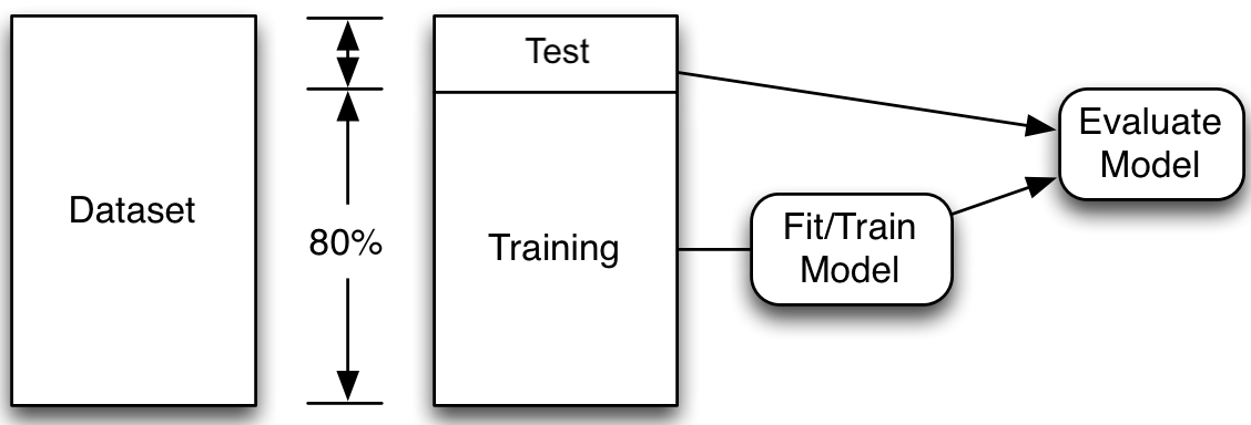
The model’s metrics on the test set are the test set error. Note, there is also the term test error which is the model’s expected (or “theoretical”) error on unseen data. So, test set error is an estimate of the test error.
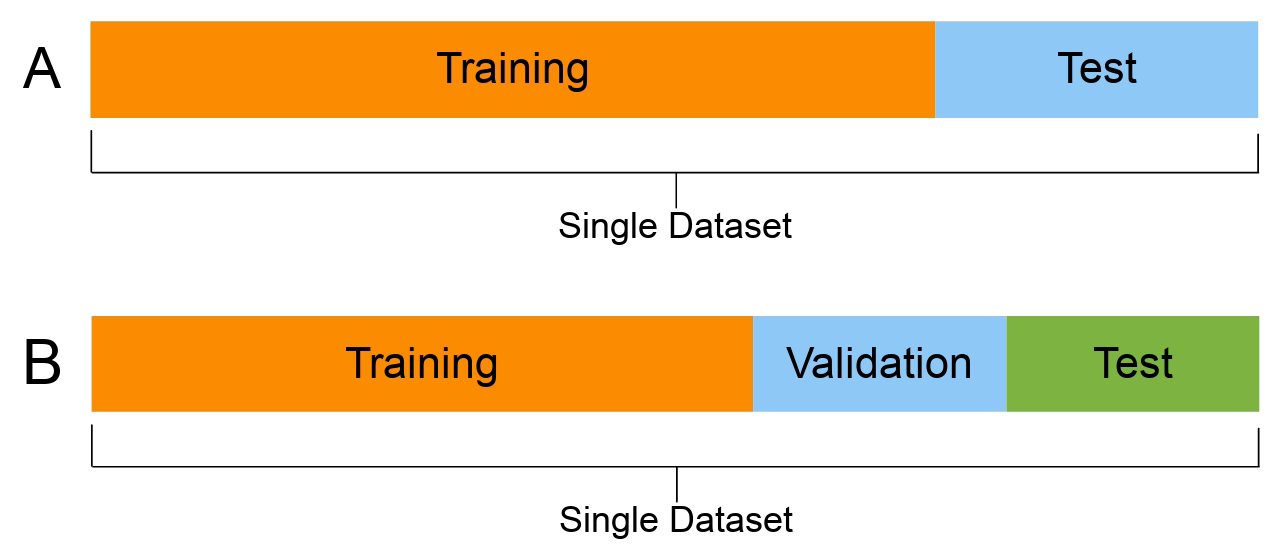
Let’s create a toy dataset where the target values are separated.
# Create a toy dataset
df_toy_classification <- data.frame(
  feature1 = c(1, 2, 3, 4, 5, 6, 7, 8, 9, 10),
  feature2 = c(2.5, 3.0, 3.9, 5.1, 6.6, 7.0, 7.5, 9.2, 10.4, 11.1),
  target = c(0, 0, 0, 0, 0, 0, 1, 1, 1, 1)
)
train_toy <- df_toy_classification[1:6, ]
test_toy <- df_toy_classification[7:10, ]train_toy# A tibble: 6 × 3
feature1 feature2 target
<dbl> <dbl> <dbl>
1 1 2.5 0
2 2 3 0
3 3 3.9 0
4 4 5.1 0
5 5 6.6 0
6 6 7 0test_toy# A tibble: 4 × 3
feature1 feature2 target
<dbl> <dbl> <dbl>
1 7 7.5 1
2 8 9.2 1
3 9 10.4 1
4 10 11.1 1model <- glm(target ~ ., data = train_toy, family = binomial)
coef(model) (Intercept) feature1 feature2
-2.456607e+01 3.407736e-16 4.777200e-16 predict(model, newdata = test_toy, type = "response") 7 8 9 10
2.143345e-11 2.143345e-11 2.143345e-11 2.143345e-11 df_toy <- data.frame(thing = c("croissant", "coffee", "gadgets", "books", "music"),
cost = c(9, 5, 100, 20, 40))Using the sample function:
set.seed(1)
sample(df_toy$thing, 3)
[1] "croissant" "books" "gadgets" You can use 1:nrow(df_toy) to get all the possible indices of the data frame.
three_indices <- sample(1:nrow(df_toy), 3)
three_indices
[1] 1 2 5df_toy[three_indices, ]# A tibble: 3 × 2
thing cost
<chr> <dbl>
1 croissant 9
2 coffee 5
3 music 40df_toy[-three_indices, ]# A tibble: 2 × 2
thing cost
<chr> <dbl>
1 gadgets 100
2 books 20# First extract the test dataset:
set.seed(1)
test_index <- sample(1:nrow(df_uni), 0.2 * nrow(df_uni))
test <- df_uni[test_index, ]
train_val <- df_uni[-test_index, ]
# Then split the rest into validation and training sets:
val_index <- sample(1:nrow(train_val), 0.25 * nrow(train_val))
val <- train_val[val_index, ]
train <- train_val[-val_index, ]dim(train)[1] 7275 18dim(val)[1] 2425 18dim(test)[1] 2424 18Remember, models tend to improve with more data (not always!).
Train on training set:
model_subrankings <- lm(overall_rating ~ work_life_balance + culture_values +
        career_opp + comp_benefits + senior_mgmt, data = train)
model_recommend <- lm(overall_rating ~ recommend + ceo_approv, data = train)
As a reference point, we can compute the training mean squared error of both models (which tends to underestimate the test error):
mean((train$overall_rating - model_subrankings$fitted.values)^2)[1] 0.3432309mean((train$overall_rating - model_recommend$fitted.values)^2)[1] 0.6185301Pick the model with the lowest validation error:
val_pred_subrankings <- predict(model_subrankings, newdata = val)
mean((val$overall_rating - val_pred_subrankings)^2)
[1] 0.3465015val_pred_recommend <- predict(model_recommend, newdata = val)
mean((val$overall_rating - val_pred_recommend)^2)[1] 0.6069284Take only the selected model, and calculate the test set error:
test_pred_subrankings <- predict(model_subrankings, newdata = test)
mean((test$overall_rating - test_pred_subrankings)^2)
[1] 0.3684643In general (but not necessarily), we expect \text{training set error} < \text{validation set error} < \text{test set error}.
Thought experiment: have m classifiers: \hat{f}_1(\boldsymbol{x}), \dots, \hat{f}_m(\boldsymbol{x}).
They are just as good as each other in the long run \mathbb{P}(\, \hat{f}_i(\boldsymbol{X}) = Y \,)\ =\ 90\% , \quad \text{for } i=1,\dots,m .
Evaluate each model on the validation set, some will be better than others.
If you just took the best, you’d think it has \approx 98\% accuracy!
set.seed(2)
m <- 50
x <- rnorm(m, mean = 0.9, sd = 0.03)
data <- data.frame(x = x, y = rep(0, m))

# Combined plot with histogram
p <- ggplot(data, aes(x = x)) +
  geom_histogram(aes(y = after_stat(density)), binwidth = 0.02, fill = "blue", alpha = 0.5, color = "black") +
  geom_point(aes(y = y)) +
  geom_vline(xintercept = 0.9, linetype = "dashed", color = "black") +
  geom_vline(xintercept = max(x), linetype = "dashed", color = "red") +
  labs(x = "Accuracy of each model on validation set", y = "Count") +
  xlim(min(x) - 0.02, max(x) + 0.02) +
  theme_minimal()

print(p)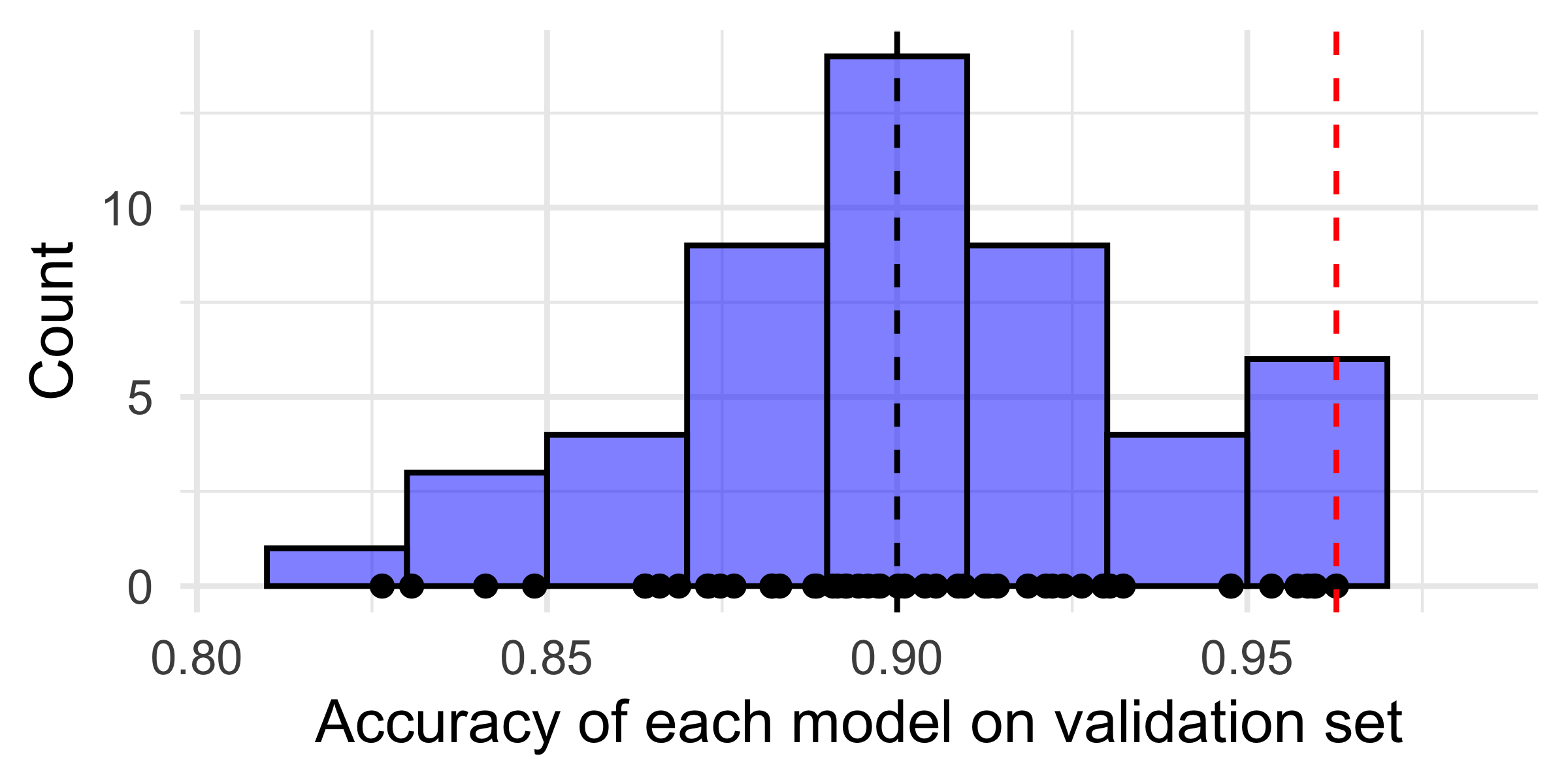
You get unbiased estimates for each model’s accuracy.
However, you get a biased estimate for the best model’s future performance.
Your best validation set model only trained on a fraction (e.g. 60%) of the data.
Retrain on the train and validation set combined (often 80%):
model_subrankings_train_val <- update(model_subrankings, data = rbind(train, val))Can still estimate the test error for this new model:
test_pred_subrankings_train_val <- predict(model_subrankings_train_val, newdata = test)
mean((test_pred_subrankings_train_val - test$overall_rating)^2)
[1] 0.3686027Lastly, if you want the best possible model, you can retrain on the entire dataset:
model_subrankings_all <- update(model_subrankings, data = df_uni)But we have no unseen data to test this on!
“In statistics, sometimes we only use a single data set. To still be able to evaluate the performance of the developed prediction model on the same data, sophisticated methods have developed over a long period of time and are still in use in some parts of the statistics community. These methods account for the fact that the model saw the data during fitting and applied corrections to account for that. These methods include, for example, the Akaike Information Criterion (AIC) or the Bayesian Information Criterion (BIC). Don’t get confused. If you have a validation set, you don’t need these methods.”
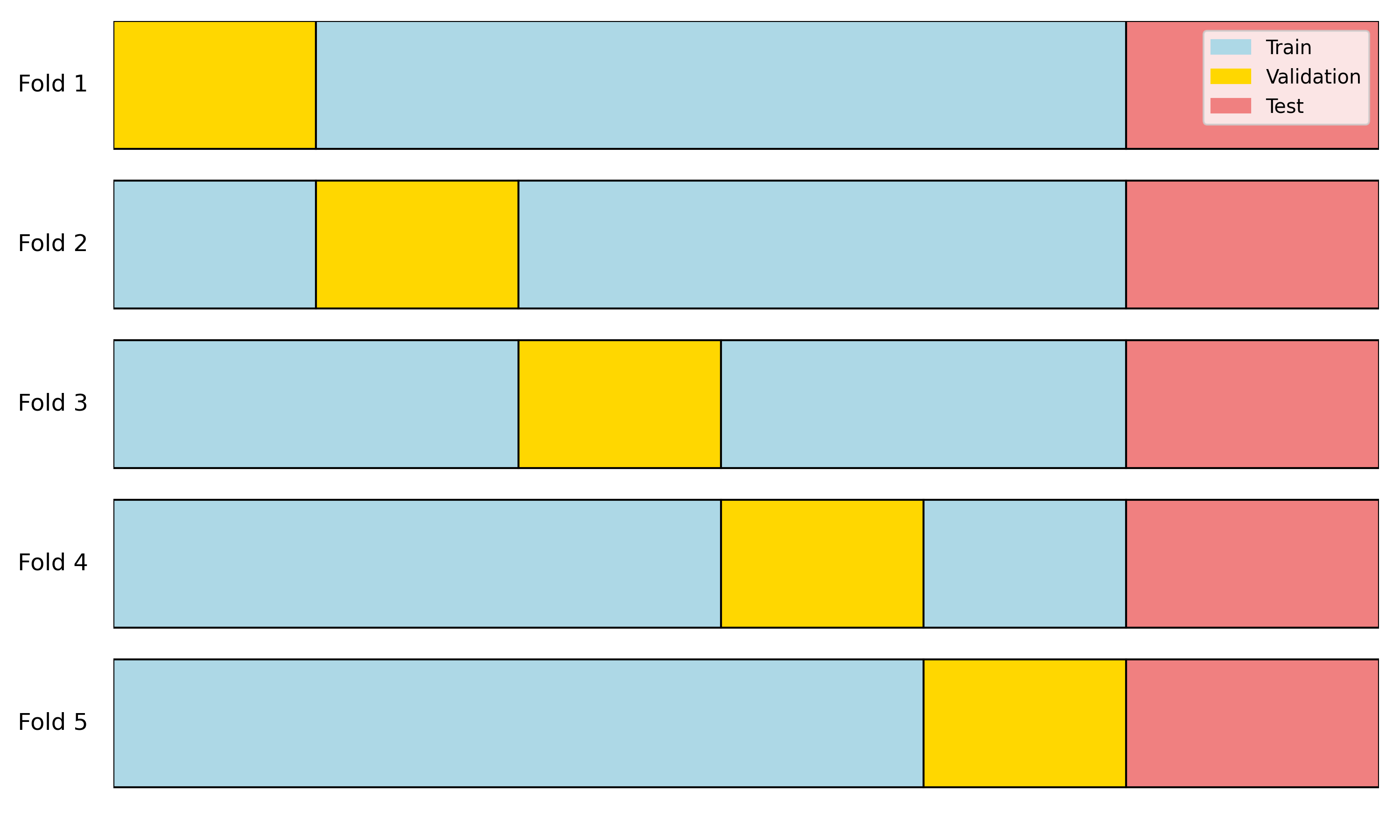
set.seed(123)
train_val <- rbind(train, val)
train_val_shuffle <- train_val[sample(1:nrow(train_val)), ]
k <- 5
fold_size <- floor(nrow(train_val) / k)
mse_subrankings <- numeric(k)
mse_recommend <- numeric(k)

for (i in 1:k) {
  val_indices <- ((i - 1) * fold_size + 1):(i * fold_size)
  val <- train_val_shuffle[val_indices, ]
  train <- train_val_shuffle[-val_indices, ]

  model_subrankings <- lm(overall_rating ~ work_life_balance + culture_values +
                            career_opp + comp_benefits + senior_mgmt, data = train)
  model_recommend <- lm(overall_rating ~ recommend + ceo_approv, data = train)

  mse_subrankings[i] <- mean((predict(model_subrankings, newdata = val) - val$overall_rating)^2)
  mse_recommend[i] <- mean((predict(model_recommend, newdata = val) - val$overall_rating)^2)
}
mse_subrankings # MSEs for the 5 folds of model "subrankings"
[1] 0.3412937 0.3793135 0.3341551 0.3282538 0.3402309mse_recommend # MSEs for the 5 folds of model "recommend" [1] 0.5922074 0.6044508 0.6594366 0.6154871 0.6093461c(mean(mse_subrankings), mean(mse_recommend)) # average MSEs across folds[1] 0.3446494 0.6161856model_recommend <- lm(
overall_rating ~ recommend + ceo_approv,
data = train_val)
summary(model_recommend)
Call:
lm(formula = overall_rating ~ recommend + ceo_approv, data = train_val)

Residuals:
    Min      1Q  Median      3Q     Max
-3.5685 -0.5558 -0.0595  0.6046  3.0133

Coefficients:
                   Estimate Std. Error t value Pr(>|t|)
(Intercept)         4.05949    0.01757 231.037  < 2e-16 ***
recommendPositive   0.33592    0.02415  13.911  < 2e-16 ***
recommendNegative  -1.50366    0.03262 -46.097  < 2e-16 ***
ceo_approvPositive  0.17313    0.02291   7.557 4.48e-14 ***
ceo_approvMild     -0.18049    0.02298  -7.853 4.50e-15 ***
ceo_approvNegative -0.56915    0.03921 -14.516  < 2e-16 ***
---
Signif. codes:  0 '***' 0.001 '**' 0.01 '*' 0.05 '.' 0.1 ' ' 1

Residual standard error: 0.7848 on 9694 degrees of freedom
Multiple R-squared:  0.4366,    Adjusted R-squared:  0.4363
F-statistic:  1503 on 5 and 9694 DF,  p-value: < 2.2e-16
model_recommend <- glm(
overall_rating ~ recommend + ceo_approv,
data = train_val)
summary(model_recommend)
Call:
glm(formula = overall_rating ~ recommend + ceo_approv, data = train_val)

Coefficients:
                   Estimate Std. Error t value Pr(>|t|)
(Intercept)         4.05949    0.01757 231.037  < 2e-16 ***
recommendPositive   0.33592    0.02415  13.911  < 2e-16 ***
recommendNegative  -1.50366    0.03262 -46.097  < 2e-16 ***
ceo_approvPositive  0.17313    0.02291   7.557 4.48e-14 ***
ceo_approvMild     -0.18049    0.02298  -7.853 4.50e-15 ***
ceo_approvNegative -0.56915    0.03921 -14.516  < 2e-16 ***
---
Signif. codes:  0 '***' 0.001 '**' 0.01 '*' 0.05 '.' 0.1 ' ' 1

(Dispersion parameter for gaussian family taken to be 0.6159165)

    Null deviance: 10597.8  on 9699  degrees of freedom
Residual deviance:  5970.7  on 9694  degrees of freedom
AIC: 22834

Number of Fisher Scoring iterations: 2cv.glmNo need to write your own loop, you can use a function like cv.glm:
library(boot)

set.seed(123)

# Fit the models as 'glm's first
model_subrankings <- glm(overall_rating ~ work_life_balance + culture_values + career_opp +
    comp_benefits + senior_mgmt, data = train_val)
model_recommend <- glm(overall_rating ~ recommend + ceo_approv, data = train_val)

# Pass them to 'cv.glm'
cv_subrankings <- cv.glm(train_val, model_subrankings, K = 5)
cv_recommend <- cv.glm(train_val, model_recommend, K = 5)

(cv_mse_subrankings <- cv_subrankings$delta[1])
[1] 0.3447204(cv_mse_recommend <- cv_recommend$delta[1])[1] 0.6168303Discuss how you expect LOOCV to perform relative to the Validation Set approach. Any obvious pros and/or cons?
(movies <- read.csv("Movies.csv"))# A tibble: 8 × 6
Movie.ID Movie.Title Release.Year Runtime Budget Box.Office
<int> <chr> <int> <int> <chr> <chr>
1 1 Harry Potter and the Philosop… 2001 152 "$125… "$1,002,0…
2 2 Harry Potter and the Chamber … 2002 161 "$100… "$880,300…
3 3 Harry Potter and the Prisoner… 2004 142 "$130… "$796,700…
4 4 Harry Potter and the Goblet o… 2005 157 "$150… "$896,400…
5 5 Harry Potter and the Order of… 2007 138 "$150… "$942,000…
6 6 Harry Potter and the Half-Blo… 2009 153 "$250… "$943,200…
7 7 Harry Potter and the Deathly … 2010 146 "$200… "$976,900…
8 8 Harry Potter and the Deathly … 2011 130 "$250… "$1,342,0…# Clean the dataset and convert relevant columns to numerical format
movies$Budget <- as.numeric(gsub("[\\$,]", "", movies$Budget))
movies$Box.Office <- as.numeric(gsub("[\\$,]", "", movies$Box.Office))# Grab just one movie as a test set
set.seed(1)
test_index <- sample(1:nrow(movies), 1)
train_val <- movies[-test_index, ]
(test <- movies[test_index, ])# A tibble: 1 × 6
Movie.ID Movie.Title Release.Year Runtime Budget Box.Office
<int> <chr> <int> <int> <dbl> <dbl>
1 1 Harry Potter and the Philosop… 2001 152 1.25e8 1002000000model_year <- glm(Box.Office ~ Budget + Release.Year, data = train_val)
model_runtime <- glm(Box.Office ~ Budget + Runtime, data = train_val)
cv_year <- cv.glm(train_val, model_year) # cv.glm defaults to LOOCV
cv_runtime <- cv.glm(train_val, model_runtime)cv_year$delta[1][1] 5.76601e+16cv_runtime$delta[1][1] 4.987983e+16# Test error for the runtime model
test_pred_runtime <- predict(model_runtime, newdata = test)
(mean((test$Box.Office - test_pred_runtime)^2))[1] 2.147352e+16summary(model_runtime)$coefficients Estimate Std. Error t value Pr(>|t|)
(Intercept) 1.654606e+09 8.864632e+08 1.866526 0.1353742
Budget 1.543067e+00 1.011329e+00 1.525781 0.2017612
Runtime -6.526499e+06 5.404189e+06 -1.207674 0.2936943# Load dataset
library(mlbench)
data(BostonHousing)
# Split the data into training and test sets
set.seed(123)
train_index <- sample(nrow(BostonHousing),
0.8 * nrow(BostonHousing))
train <- BostonHousing[train_index, ]
test <- BostonHousing[-train_index, ]
# Fit a linear regression model
lm_model <- lm(medv ~ ., data = train)
# Calculate the training and test errors
train_pred <- predict(lm_model, newdata = train)
train_error <- mean((train_pred - train$medv)^2)
lm_model <- lm(medv ~ ., data = test)
test_pred <- predict(lm_model, newdata = test)
test_error <- mean((test_pred - test$medv)^2)
# Print the training and test errors
cat("Training Error (MSE):", train_error, "\n")Training Error (MSE): 21.60875 cat("Test Error (MSE):", test_error, "\n")Test Error (MSE): 20.26994 3a) Which do you expect to be lower on average, the training loss or the test loss? Why?
3b) Describe why, in this case, the test error is less than the training error.
Model has been re-trained on the test set for the purpose of computing the “test error”… this is illegal!

Traditional linear regression methods

Traditional methods break, regularisation methods can help
If p > n, \text{R} will just fit the first n parameters and give NA for the rest.
first_few_rows <- df_uni[1:3, ]
model_subrankings <- lm(overall_rating ~ work_life_balance + culture_values +
        career_opp + comp_benefits + senior_mgmt, data = first_few_rows)
summary(model_subrankings)
Call:
lm(formula = overall_rating ~ work_life_balance + culture_values +
    career_opp + comp_benefits + senior_mgmt, data = first_few_rows)

Residuals:
ALL 3 residuals are 0: no residual degrees of freedom!

Coefficients: (3 not defined because of singularities)
                  Estimate Std. Error t value Pr(>|t|)
(Intercept)         3.6667        NaN     NaN      NaN
work_life_balance  -0.3333        NaN     NaN      NaN
culture_values      0.6667        NaN     NaN      NaN
career_opp              NA         NA      NA       NA
comp_benefits           NA         NA      NA       NA
senior_mgmt             NA         NA      NA       NA

Residual standard error: NaN on 0 degrees of freedom
Multiple R-squared:      1, Adjusted R-squared:    NaN
F-statistic: NaN on 2 and 0 DF, p-value: NAMinimise the following (for \boldsymbol{\beta}):
\sum_{i=1}^n \Bigl( y_i - \beta_0 - \sum_{j=1}^p \beta_jx_{ij} \Bigr)^2 + \lambda \sum_{j=1}^p \beta^2_j = \text{RSS} + \lambda \sum_{j=1}^p \beta^2_j
Minimise the following (for \boldsymbol{\beta}):
\sum_{i=1}^n \Bigl( y_i - \beta_0 - \sum_{j=1}^p \beta_jx_{ij} \Bigr)^2 + \lambda \sum_{j=1}^p |\beta_j| = \text{RSS} + \lambda \sum_{j=1}^p |\beta_j|
glmnet() we use for ridge & lasso regression will do this for us (by default).Combines ridge and lasso penalties, so you minimise
\text{RSS} + \lambda \Bigl[ \, \alpha \sum_{j=1}^p |\beta_j| + (1-\alpha) \sum_{j=1}^p \beta_j^2 \, \Bigr]
glmnet package fits elastic net models, so you have to choose \alpha=0 or \alpha=1 to get ridge or lasso.glmnet package.\boldsymbol{\beta}_\text{LM} = (\boldsymbol{X}^\top\boldsymbol{X})^{-1} \boldsymbol{X}^\top \boldsymbol{y}
model_subrankings <- lm(overall_rating ~ work_life_balance + culture_values + career_opp + comp_benefits + senior_mgmt, data = first_few_rows)
coef(model_subrankings)
(Intercept) work_life_balance culture_values career_opp
3.6666667 -0.3333333 0.6666667 NA
comp_benefits senior_mgmt
NA NA X <- model.matrix(~ work_life_balance + culture_values + career_opp + comp_benefits + senior_mgmt, data = first_few_rows)
X <- cbind(rep(1, nrow(X)), scale(X[, -1])) # Scale the columns (apart from intercept)
y <- first_few_rows$overall_rating
beta <- solve(t(X) %*% X) %*% t(X) %*% yError in solve.default(t(X) %*% X): Lapack routine dgesv: system is exactly singular: U[6,6] = 0\boldsymbol{\beta}_{\text{Ridge}} = (\boldsymbol{X}^\top\boldsymbol{X} + \lambda\boldsymbol{I})^{-1} \boldsymbol{X}^\top \boldsymbol{y}
ridge <- glmnet(X[,-1], y, alpha = 0, lambda=0.01, standardize=F)
coef(ridge, s=0.01)
6 x 1 sparse Matrix of class "dgCMatrix"
s1
(Intercept) 4.33333333
work_life_balance -0.02281223
culture_values 0.12935580
career_opp 0.15756346
comp_benefits 0.17078714
senior_mgmt -0.15731707beta <- solve(t(X) %*% X + 0.01 * diag(ncol(X))) %*% t(X) %*% y
beta [,1]
4.3189369
work_life_balance -0.0252433
culture_values 0.1338977
career_opp 0.1591410
comp_benefits 0.1691859
senior_mgmt -0.1581698set.seed(4)
x <- rnorm(50)
y <- x - 2*x^2 + rnorm(100)
data <- data.frame(x = x, y = y)
# Generate true curve
x_grid <- seq(min(x), max(x), length=500)
y_true <- x_grid - 2*x_grid^2
true_curve <- data.frame(x = x_grid, y = y_true)
# Plot the data with the true curve
ggplot(data, aes(x = x, y = y)) +
geom_point() +
geom_line(data = true_curve, aes(x = x, y = y), color = "green") +
labs(x = "x", y = "y") +
theme_minimal()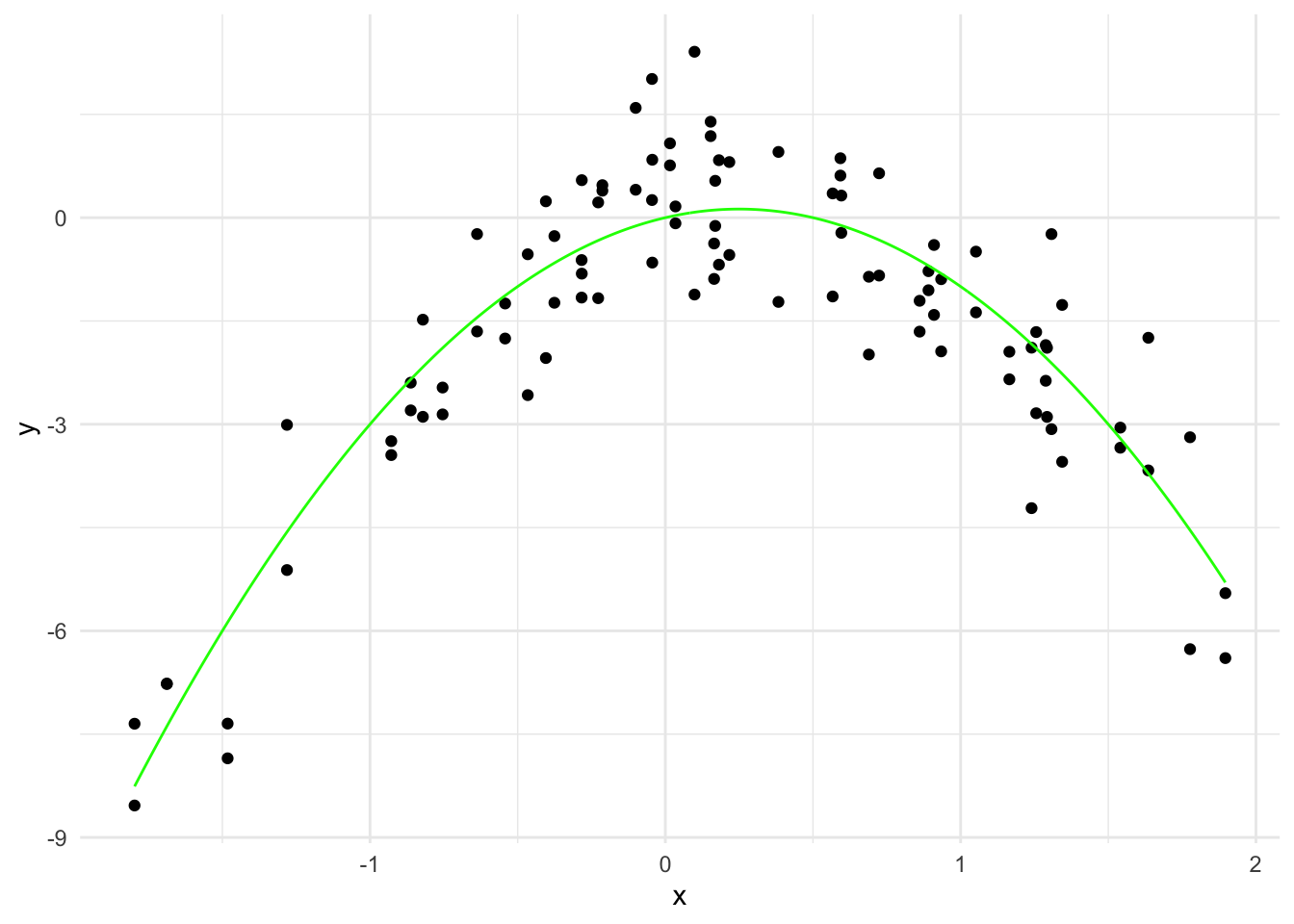
# Fit a linear model
linear_model <- lm(y ~ poly(x, 20, raw=TRUE), data = data)

# Generate predictions over the data
y_hat <- predict(linear_model, data.frame(x = x_grid))
linear_predictions <- data.frame(x = x_grid, y = y_hat)

ggplot(data, aes(x = x, y = y)) +
  geom_point() +
  geom_line(data = true_curve, aes(x = x, y = y), color = "green") +
  geom_line(data = linear_predictions, aes(x = x, y = y), color = "red") +
  labs(x = "x", y = "y") +
  theme_minimal()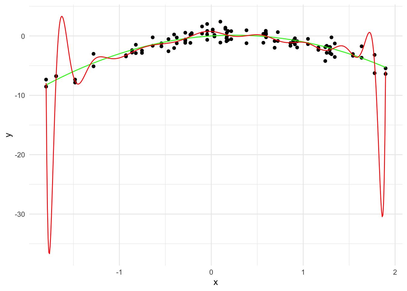
\hat{y}(x) = 0.76 - 1.09 x - 22.91 x^2 + \cdots - 1.77 x^{19} + 2.15 x^{20}
The \sum_{j=1}^{20} \hat{\beta}_j^2 is 6970618.
# Create a data frame with the predictors
x_poly <- model.matrix(~ poly(x, 20, raw=TRUE), data = data)[, -1]
x_grid_poly <- model.matrix(~ poly(x_grid, 20, raw=TRUE))[, -1]
colnames(x_grid_poly) <- colnames(x_poly)

ridge_model <- glmnet(x_poly, y, alpha = 0, lambda=c(0.01, 0.1, 1, 10))

# Generate predictions over the data
y_hat <- predict(ridge_model, newx=x_grid_poly, s = 0.01)
linear_predictions <- data.frame(x = x_grid, y = y_hat)
names(linear_predictions) <- c("x", "y")

ggplot(data, aes(x = x, y = y)) +
  geom_point() +
  geom_line(data = true_curve, aes(x = x, y = y), color = "green") +
  geom_line(data = linear_predictions, aes(x = x, y = y), color = "red") +
  labs(x = "x", y = "y") +
  theme_minimal()
\hat{y}(x) = 0.20 + 0.92 x - 2.73 x^2 + \cdots + 0.000007 x^{19} - 0.000003 x^{20}
The \sum_{j=1}^{20} \hat{\beta}_j^2 is 8.31.
y_hat_0_1 <- predict(ridge_model, x_grid_poly, s = 0.1)
ridge_predictions_0_1 <- data.frame(x = x_grid, y = y_hat_0_1)
names(ridge_predictions_0_1) <- c("x", "y")

ggplot(data, aes(x = x, y = y)) +
  geom_point() +
  geom_line(data = true_curve, aes(x = x, y = y), color = "green") +
  geom_line(data = ridge_predictions_0_1, aes(x = x, y = y), color = "blue") +
  labs(x = "x", y = "y") +
  theme_minimal()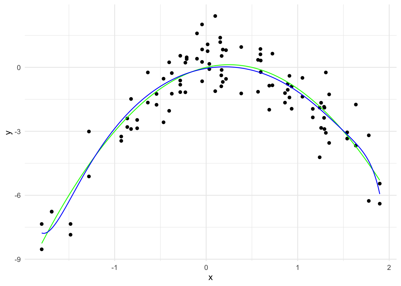
\hat{y}(x) = -0.05 + 0.73 x - 1.82 x^2 + \cdots - 0.000004 x^{19} - 0.000001 x^{20}
The \sum_{j=1}^{20} \hat{\beta}_j^2 is 3.86.
y_hat_1 <- predict(ridge_model, x_grid_poly, s = 1)
ridge_predictions_1 <- data.frame(x = x_grid, y = y_hat_1)
names(ridge_predictions_1) <- c("x", "y")

ggplot(data, aes(x = x, y = y)) +
  geom_point() +
  geom_line(data = true_curve, aes(x = x, y = y), color = "green") +
  geom_line(data = ridge_predictions_1, aes(x = x, y = y), color = "blue") +
  labs(x = "x", y = "y") +
  theme_minimal()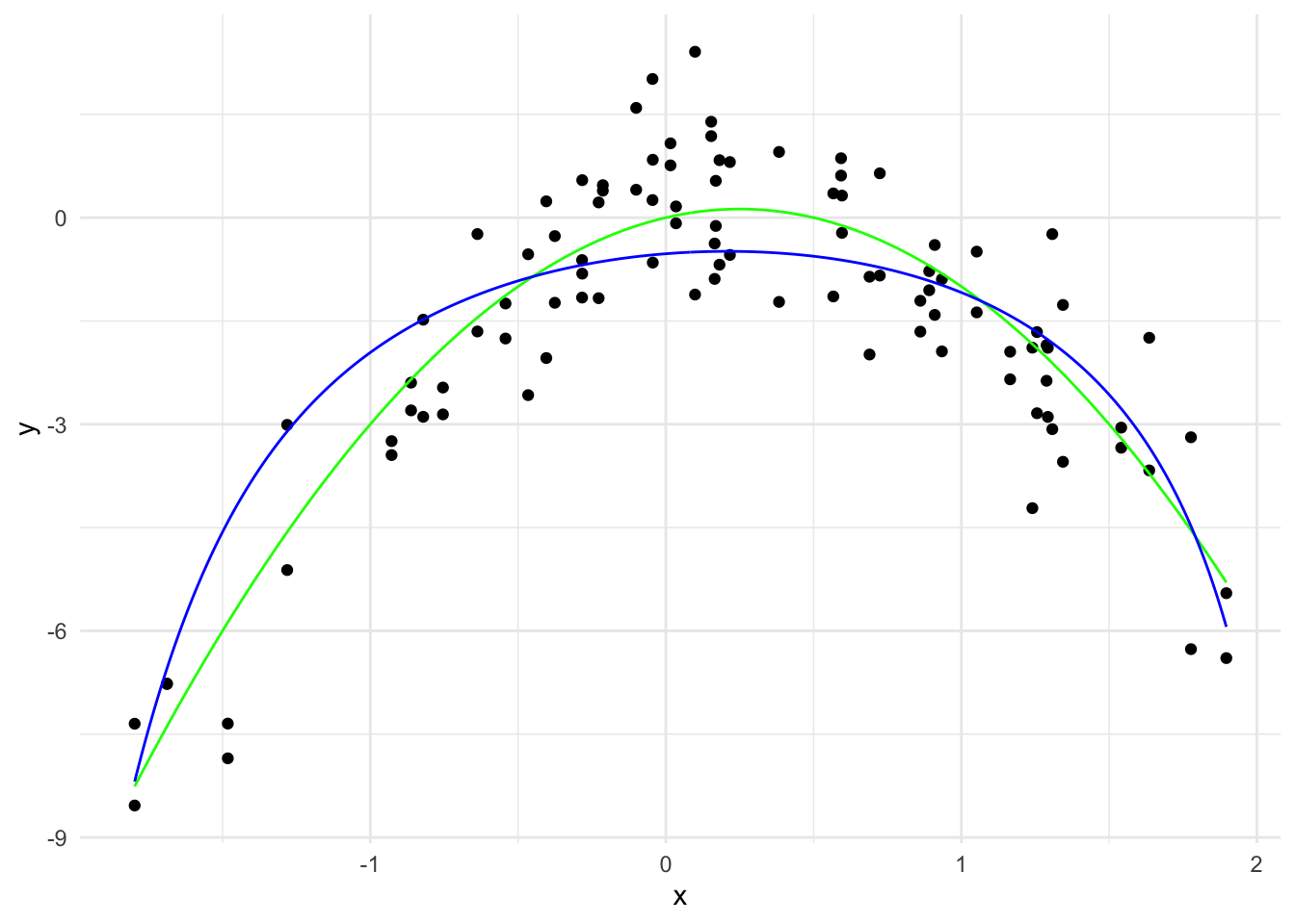
\hat{y}(x) = -0.52 + 0.34 x - 0.82 x^2 + \cdots - 0.0000006 x^{19} + 0.00000007 x^{20}
The \sum_{j=1}^{20} \hat{\beta}_j^2 is 0.818.
y_hat_10 <- predict(ridge_model, x_grid_poly, s = 10)
ridge_predictions_10 <- data.frame(x = x_grid, y = y_hat_10)
names(ridge_predictions_10) <- c("x", "y")

ggplot(data, aes(x = x, y = y)) +
  geom_point() +
  geom_line(data = true_curve, aes(x = x, y = y), color = "green") +
  geom_line(data = ridge_predictions_10, aes(x = x, y = y), color = "blue") +
  labs(x = "x", y = "y") +
  theme_minimal()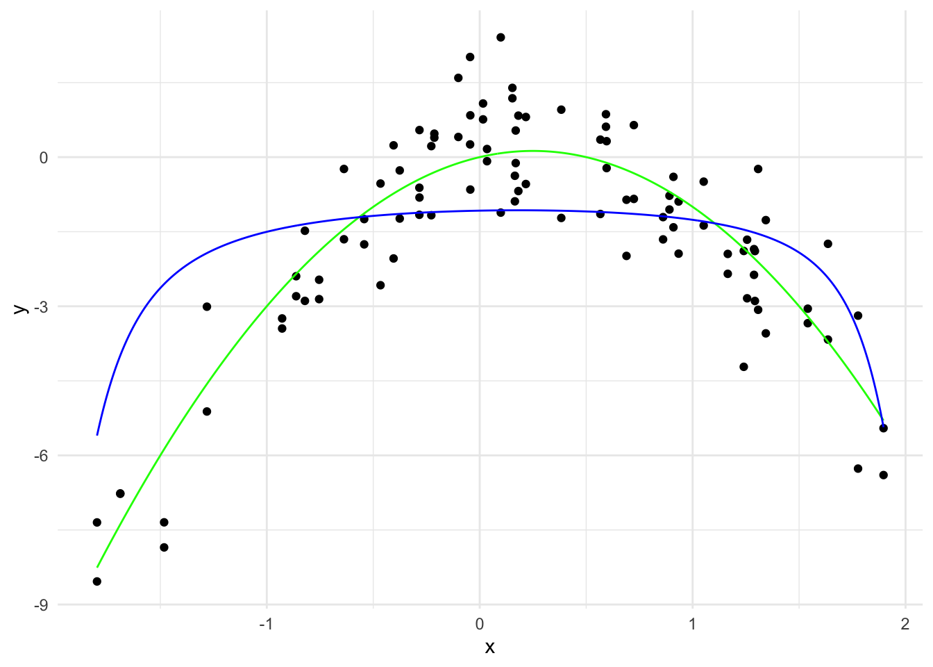
\hat{y}(x) = -1.08 + 0.08 x - 0.23 x^2 + \cdots + 0.0000003 x^{19} - 0.000001 x^{20}
The \sum_{j=1}^{20} \hat{\beta}_j^2 is 0.0624.
ridge_model <- glmnet(x_poly, y, alpha=0)
plot(ridge_model, xvar="lambda", label=TRUE)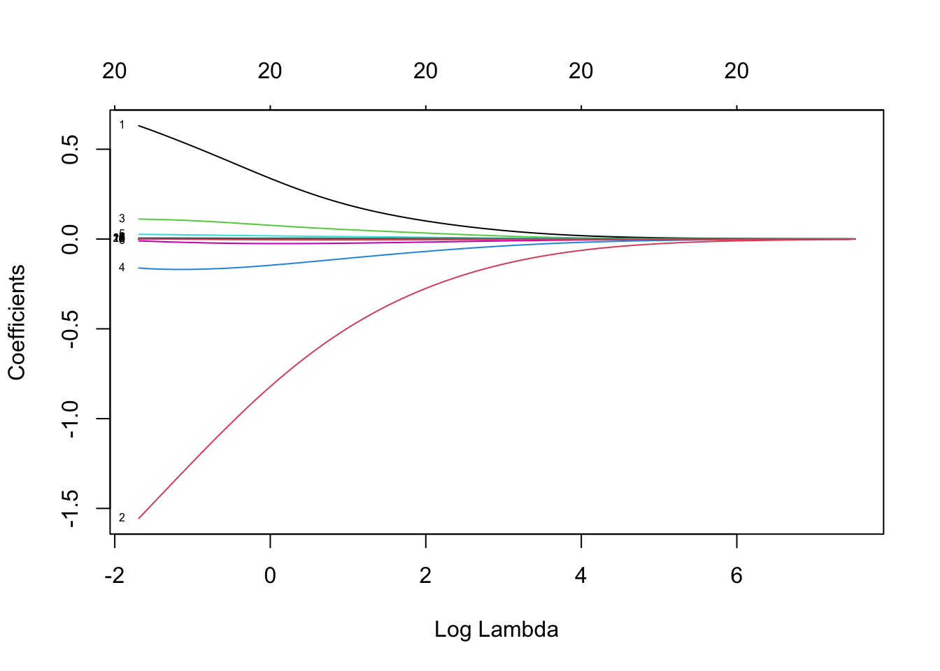
# Find the best lambda
cv_out <- cv.glmnet(x_poly, y, alpha = 0, nfolds=10)
plot(cv_out)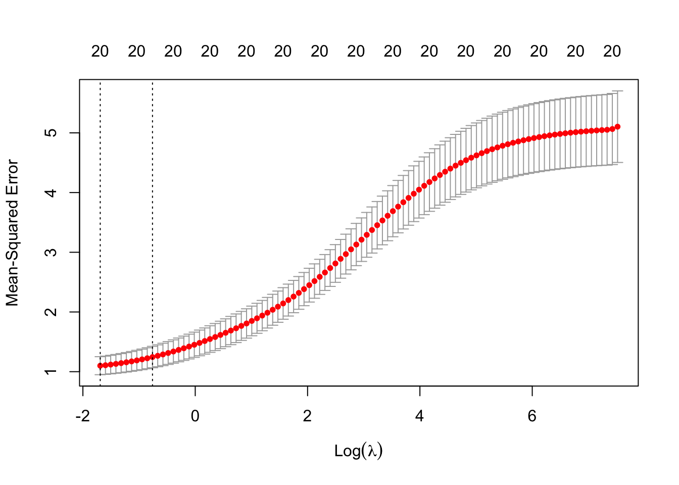
The \lambda which minimises the 10-fold CV MSE is 0.1842555 (\log(\lambda) is -1.6914321).
lasso_model <- glmnet(x_poly, y, alpha = 1, lambda=c(0.01, 0.1, 1, 10))

# Generate predictions over the data
y_hat <- predict(lasso_model, newx=x_grid_poly, s = 0.01)
linear_predictions <- data.frame(x = x_grid, y = y_hat)
names(linear_predictions) <- c("x", "y")

ggplot(data, aes(x = x, y = y)) +
  geom_point() +
  geom_line(data = true_curve, aes(x = x, y = y), color = "green") +
  geom_line(data = linear_predictions, aes(x = x, y = y), color = "red") +
  labs(x = "x", y = "y") +
  theme_minimal()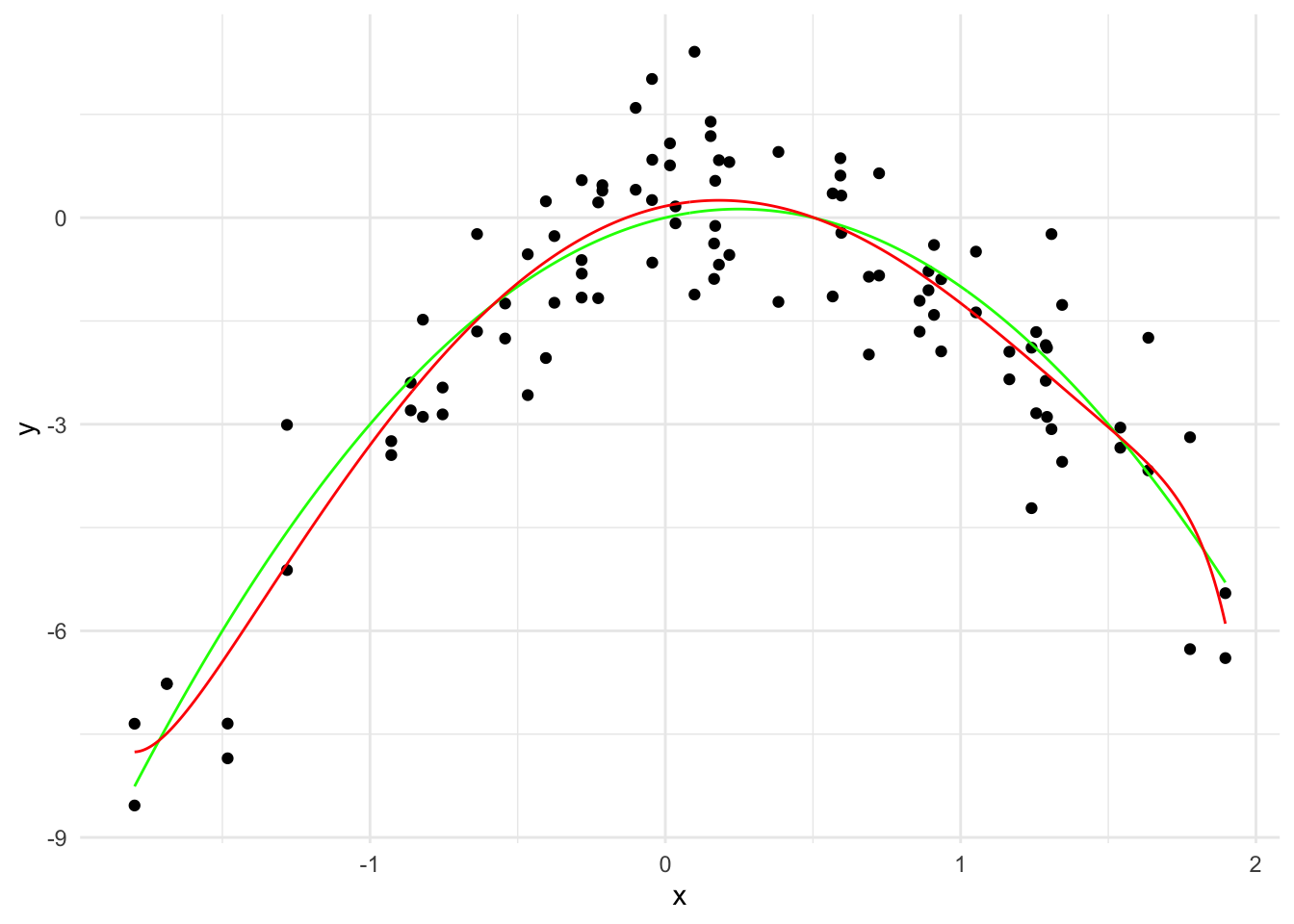
\hat{y}(x) = 0.17 + 0.93 x - 2.60 x^2 + \cdots - 3.29 \times 10^{-6} x^{19} - 5.95 \times 10^{-7} x^{20}
The \sum_{j=1}^{20} |\hat{\beta}_j| is 3.79 and there are 8 non-zero coefficients.
y_hat_0_1 <- predict(lasso_model, x_grid_poly, s = 0.1)
lasso_predictions_0_1 <- data.frame(x = x_grid, y = y_hat_0_1)
names(lasso_predictions_0_1) <- c("x", "y")

ggplot(data, aes(x = x, y = y)) +
  geom_point() +
  geom_line(data = true_curve, aes(x = x, y = y), color = "green") +
  geom_line(data = lasso_predictions_0_1, aes(x = x, y = y), color = "blue") +
  labs(x = "x", y = "y") +
  theme_minimal()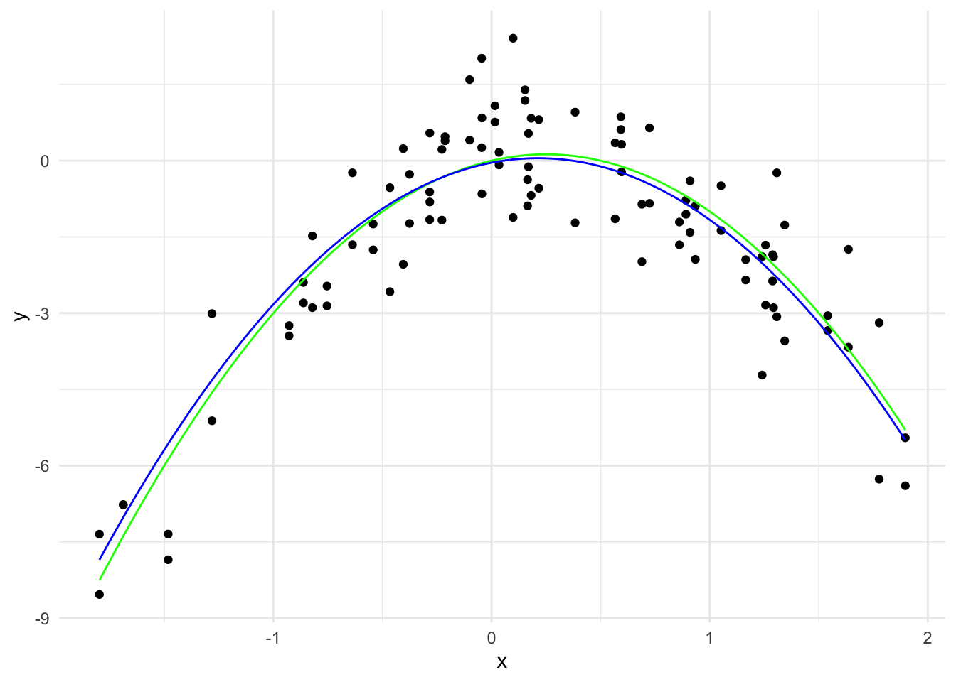
\hat{y}(x) = -0.04 + 0.83 x - 1.96 x^2
The \sum_{j=1}^{20} |\hat{\beta}_j| is 2.79 and there are 2 non-zero coefficients.
y_hat_1 <- predict(lasso_model, x_grid_poly, s = 1)
lasso_predictions_1 <- data.frame(x = x_grid, y = y_hat_1)
names(lasso_predictions_1) <- c("x", "y")

ggplot(data, aes(x = x, y = y)) +
  geom_point() +
  geom_line(data = true_curve, aes(x = x, y = y), color = "green") +
  geom_line(data = lasso_predictions_1, aes(x = x, y = y), color = "blue") +
  labs(x = "x", y = "y") +
  theme_minimal()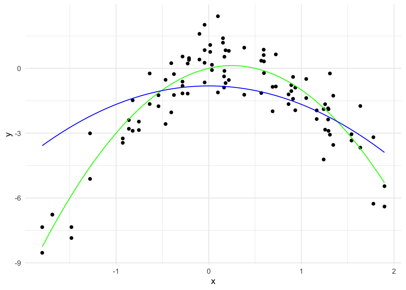
\hat{y}(x) = -0.81 - 0.86 x^2
The \sum_{j=1}^{20} |\hat{\beta}_j| is 0.855 and there are 1 non-zero coefficients.
y_hat_10 <- predict(lasso_model, x_grid_poly, s = 10)
lasso_predictions_10 <- data.frame(x = x_grid, y = y_hat_10)
names(lasso_predictions_10) <- c("x", "y")

ggplot(data, aes(x = x, y = y)) +
  geom_point() +
  geom_line(data = true_curve, aes(x = x, y = y), color = "green") +
  geom_line(data = lasso_predictions_10, aes(x = x, y = y), color = "blue") +
  labs(x = "x", y = "y") +
  theme_minimal()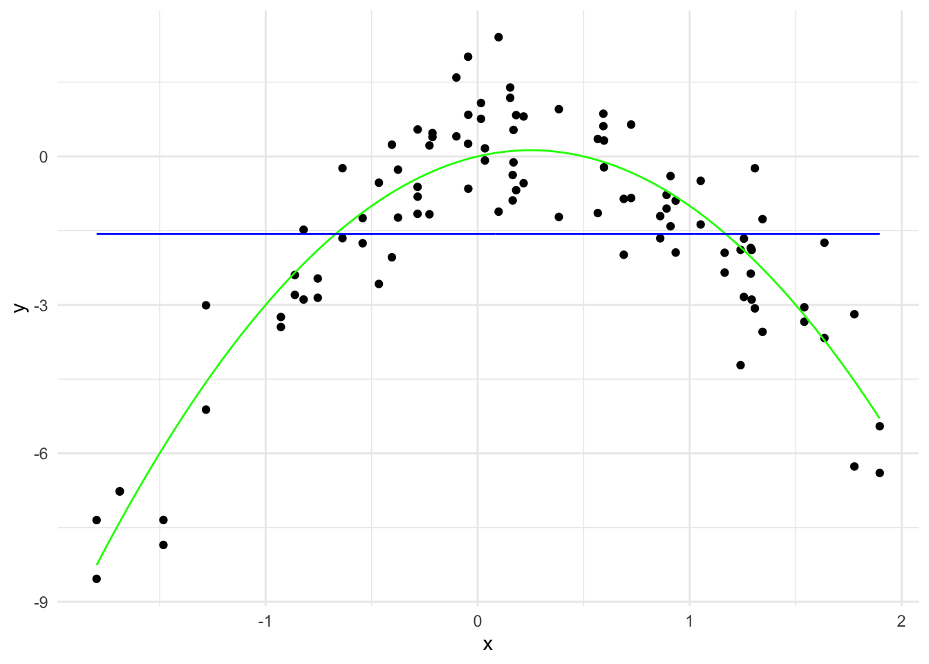
\hat{y}(x) = -1.57 - 1.90 \times 10^{-16} x^2
The \sum_{j=1}^{20} |\hat{\beta}_j| is 1.9e-16 and there is 1 non-zero coefficient.
lasso_model <- glmnet(x_poly, y, alpha=1)
plot(lasso_model, xvar="lambda", label=TRUE)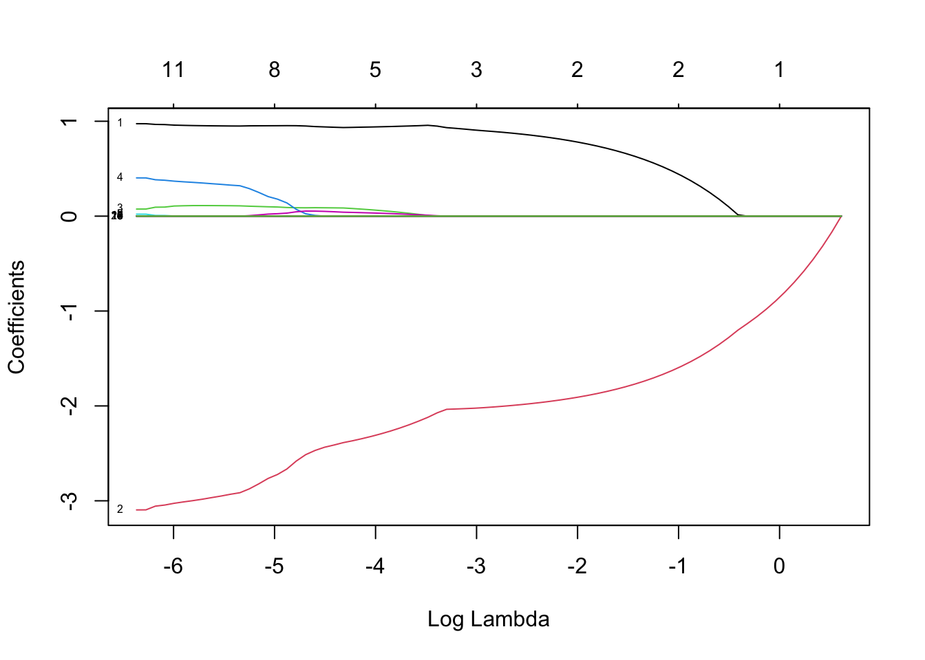
# Find the best lambda
cv_out <- cv.glmnet(x_poly, y, alpha = 1)

# Plot the cross-validated error
plot(cv_out)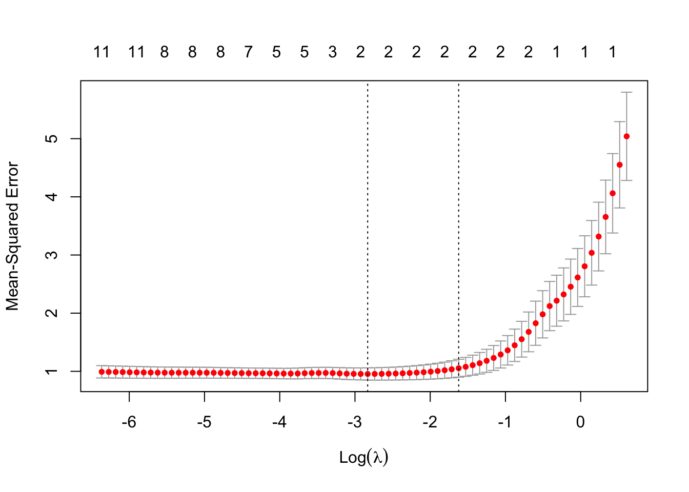
The \lambda which minimises the CV MSE is 0.0589482 (\log(\lambda) is -2.8310954).
set.seed(123)
test_index <- sample(1:nrow(df_uni), 0.2 * nrow(df_uni))
test <- df_uni[test_index, ]
train_val <- df_uni[-test_index, ]
model_subrankings <- lm(overall_rating ~ work_life_balance + culture_values +
career_opp + comp_benefits + senior_mgmt +
recommend + ceo_approv, data = train_val)
summary(model_subrankings)
Call:
lm(formula = overall_rating ~ work_life_balance + culture_values +
    career_opp + comp_benefits + senior_mgmt + recommend + ceo_approv,
    data = train_val)

Residuals:
    Min      1Q  Median      3Q     Max
-4.0109 -0.3441 -0.0248  0.3595  3.4854

Coefficients:
                    Estimate Std. Error t value Pr(>|t|)
(Intercept)         1.321466   0.032022  41.267  < 2e-16 ***
work_life_balance   0.068873   0.006287  10.954  < 2e-16 ***
culture_values      0.244629   0.007812  31.314  < 2e-16 ***
career_opp          0.175851   0.006339  27.741  < 2e-16 ***
comp_benefits       0.070892   0.006010  11.796  < 2e-16 ***
senior_mgmt         0.177644   0.007244  24.521  < 2e-16 ***
recommendPositive   0.121017   0.017635   6.862 7.19e-12 ***
recommendNegative  -0.544801   0.025401 -21.448  < 2e-16 ***
ceo_approvPositive -0.020925   0.016648  -1.257  0.20884
ceo_approvMild     -0.047943   0.016599  -2.888  0.00388 **
ceo_approvNegative -0.128851   0.028392  -4.538 5.74e-06 ***
---
Signif. codes:  0 '***' 0.001 '**' 0.01 '*' 0.05 '.' 0.1 ' ' 1

Residual standard error: 0.5638 on 9689 degrees of freedom
Multiple R-squared:  0.7169,    Adjusted R-squared:  0.7166
F-statistic:  2454 on 10 and 9689 DF,  p-value: < 2.2e-16
X <- model.matrix(overall_rating ~ work_life_balance + culture_values +
career_opp + comp_benefits + senior_mgmt +
recommend + ceo_approv, data = train_val)[,-1]
y <- train_val$overall_ratingglmnet assumes a Gaussian response (linear regression). Use argument family= to change that.ridge <- glmnet(X, y, alpha = 0)
plot(ridge, xvar="lambda", label=TRUE)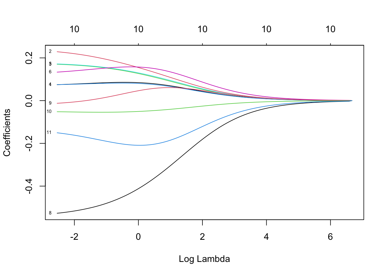
cv.glmnet does 10-fold cross-validation. Use argument nfold= to change that.cv_ridge <- cv.glmnet(X, y, alpha = 0)
plot(cv_ridge)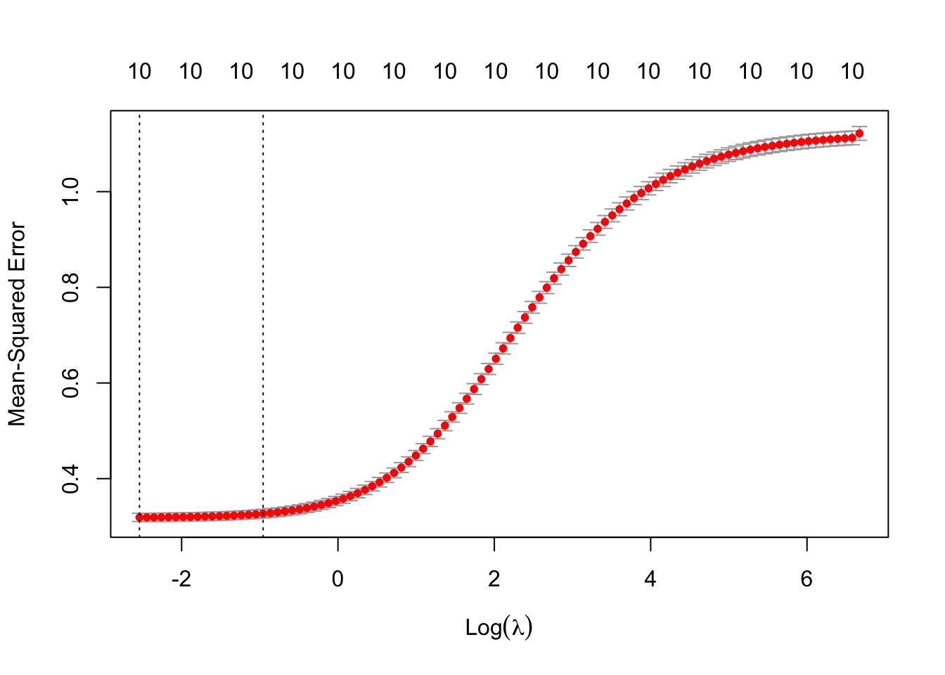
The \lambda which minimises the CV MSE is 0.0789461 (\log(\lambda) is -2.5389899).
lasso <- glmnet(X, y, alpha = 1)
plot(lasso, xvar="lambda", label=TRUE)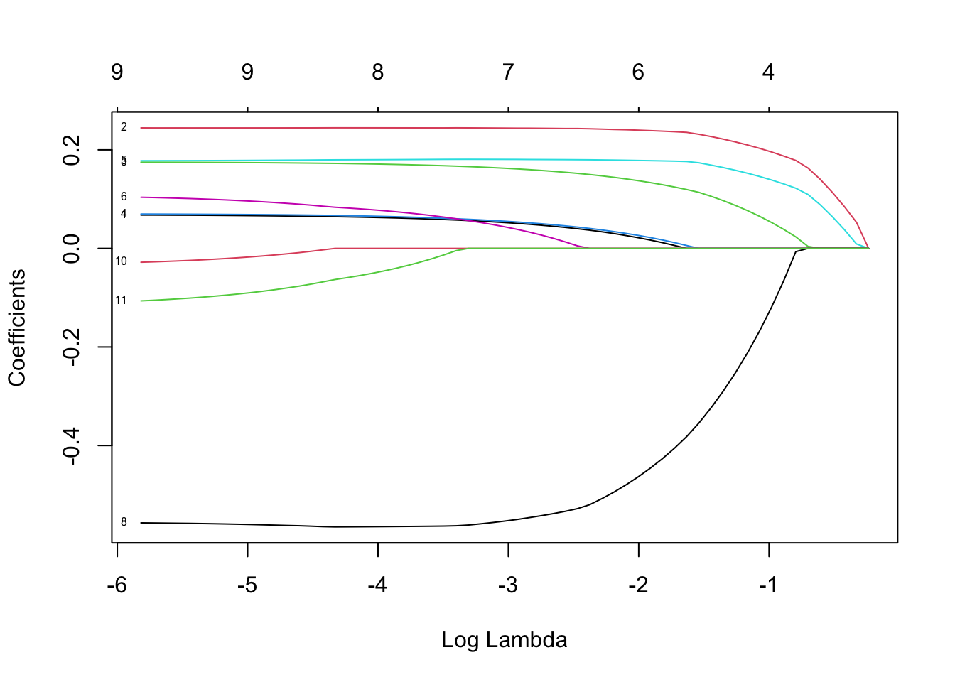
cv_lasso <- cv.glmnet(X, y, alpha = 1)
plot(cv_lasso)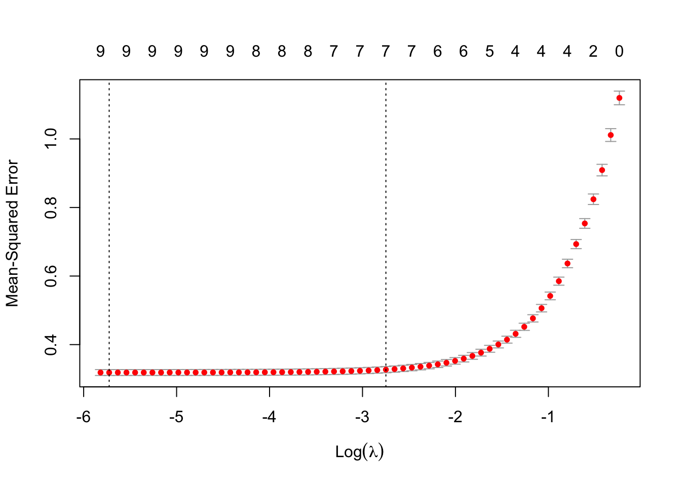
The \lambda which minimises the CV MSE is 0.0032621 (\log(\lambda) is -5.7253955).
lambda.min: the \lambda at which the smallest MSE is achieved.lambda.1se: the largest \lambda at which the MSE is within one standard error of the smallest MSE (default).coef(cv_lasso, s = "lambda.min")12 x 1 sparse Matrix of class "dgCMatrix"
s1
(Intercept) 1.33348345
work_life_balance 0.06771192
culture_values 0.24444863
career_opp 0.17493054
comp_benefits 0.06970145
senior_mgmt 0.17788762
recommendPositive 0.10325936
recommendMild .
recommendNegative -0.55711640
ceo_approvPositive .
ceo_approvMild -0.02732177
ceo_approvNegative -0.10528624coef(cv_lasso, s = "lambda.1se")12 x 1 sparse Matrix of class "dgCMatrix"
s1
(Intercept) 1.57364673
work_life_balance 0.04712771
culture_values 0.24371243
career_opp 0.15818381
comp_benefits 0.05006640
senior_mgmt 0.18033404
recommendPositive 0.02714509
recommendMild .
recommendNegative -0.54238656
ceo_approvPositive .
ceo_approvMild .
ceo_approvNegative . load_gene_data <- function() {
# Read in the information about the study participants
labels <- read.csv("2912Table2.csv", header = TRUE)
er <- labels[,14]
n <- nrow(labels)
n1 <- sum(er) # Should be 65
n2 <- n - n1 # Should be 99-65=34
# Read in the gene expressions, remove meta-info and NA rows
genes <- read.csv("2912Table3.csv", header = TRUE)
genes <- genes[ , -(1:6)]
genes <- t(as.matrix(genes[rowSums(is.na(genes)) == 0, ]))
df <- as.data.frame(genes)
df$er <- er
df
}df <- load_gene_data()
df# A tibble: 99 × 4,405
`8` `18` `20` `21` `22` `26` `27` `28` `29` `30`
<dbl> <dbl> <dbl> <dbl> <dbl> <dbl> <dbl> <dbl> <dbl> <dbl>
1 0.0164 -0.294 -0.166 0.423 -0.507 -0.559 -0.679 -0.123 -0.511 -0.837
2 -0.435 -0.270 0.0251 0.474 -0.662 -0.678 -0.0576 0.396 -0.247 -0.705
3 -0.327 -0.735 -0.0805 0.649 -0.786 -0.0397 -0.238 -0.851 -0.501 -0.820
4 0.496 -0.389 -0.121 -0.227 -0.776 0.0559 0.0206 -0.683 -0.542 -0.995
5 1.37 -0.192 -0.0716 0.265 -0.666 -0.342 0.180 -0.862 -0.386 -0.797
6 -0.191 -0.232 0.547 0.287 -0.708 -0.250 0.355 -0.0872 -0.524 -0.890
7 0.264 -0.424 0.259 1.98 -0.386 0.109 0.258 -0.749 -0.220 -0.789
8 -0.537 -0.152 0.660 0.303 -0.778 -0.791 -0.0715 -0.517 -0.299 -0.866
9 0.197 -0.292 0.173 2.17 -0.272 -0.819 -0.0359 -0.293 -0.232 -0.590
10 0.0915 -0.107 0.0381 2.44 -0.152 0.345 0.245 0.451 -0.103 -0.414
# ℹ 89 more rows
# ℹ 4,395 more variables: `32` <dbl>, `33` <dbl>, `35` <dbl>, `37` <dbl>,
# `38` <dbl>, `39` <dbl>, `40` <dbl>, `42` <dbl>, `43` <dbl>, `44` <dbl>,
# `45` <dbl>, `46` <dbl>, `49` <dbl>, `51` <dbl>, `53` <dbl>, `54` <dbl>,
# `55` <dbl>, `56` <dbl>, `57` <dbl>, `59` <dbl>, `60` <dbl>, `61` <dbl>,
# `63` <dbl>, `64` <dbl>, `65` <dbl>, `66` <dbl>, `67` <dbl>, `68` <dbl>,
# `70` <dbl>, `71` <dbl>, `72` <dbl>, `73` <dbl>, `74` <dbl>, `101` <dbl>, …“Sotiriou et al. (2003) described a breast cancer study with 99 women divided into two groups according to their oestrogen receptor status. The ER+ group (65 women) are those women where the cancer has receptors for oestrogen, and the ER− group (34 women) are those without receptors. Out of 7650 variables there are 4404 measured in all 99 samples, and we use these variables for our analysis.”
# Split and convert to matrices for `glmnet`
set.seed(123)  # For reproducibility
test_index <- sample(1:nrow(df), 0.2 * nrow(df))
test <- df[test_index, ]
train_val <- df[-test_index, ]

# Prepare data for glmnet
X <- model.matrix(er ~ ., data = train_val)[, -1]
y <- train_val$er
X_test <- model.matrix(er ~ ., data = test)[, -1]
y_test <- test$erridge_model <- glmnet(X, y, family = "binomial", alpha = 0)
plot(ridge_model, xvar="lambda")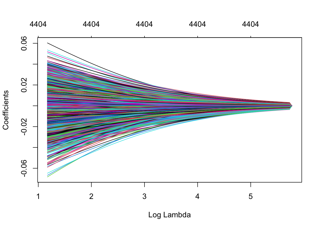
cv_ridge <- cv.glmnet(X, y, family = "binomial", alpha = 0)
plot(cv_ridge)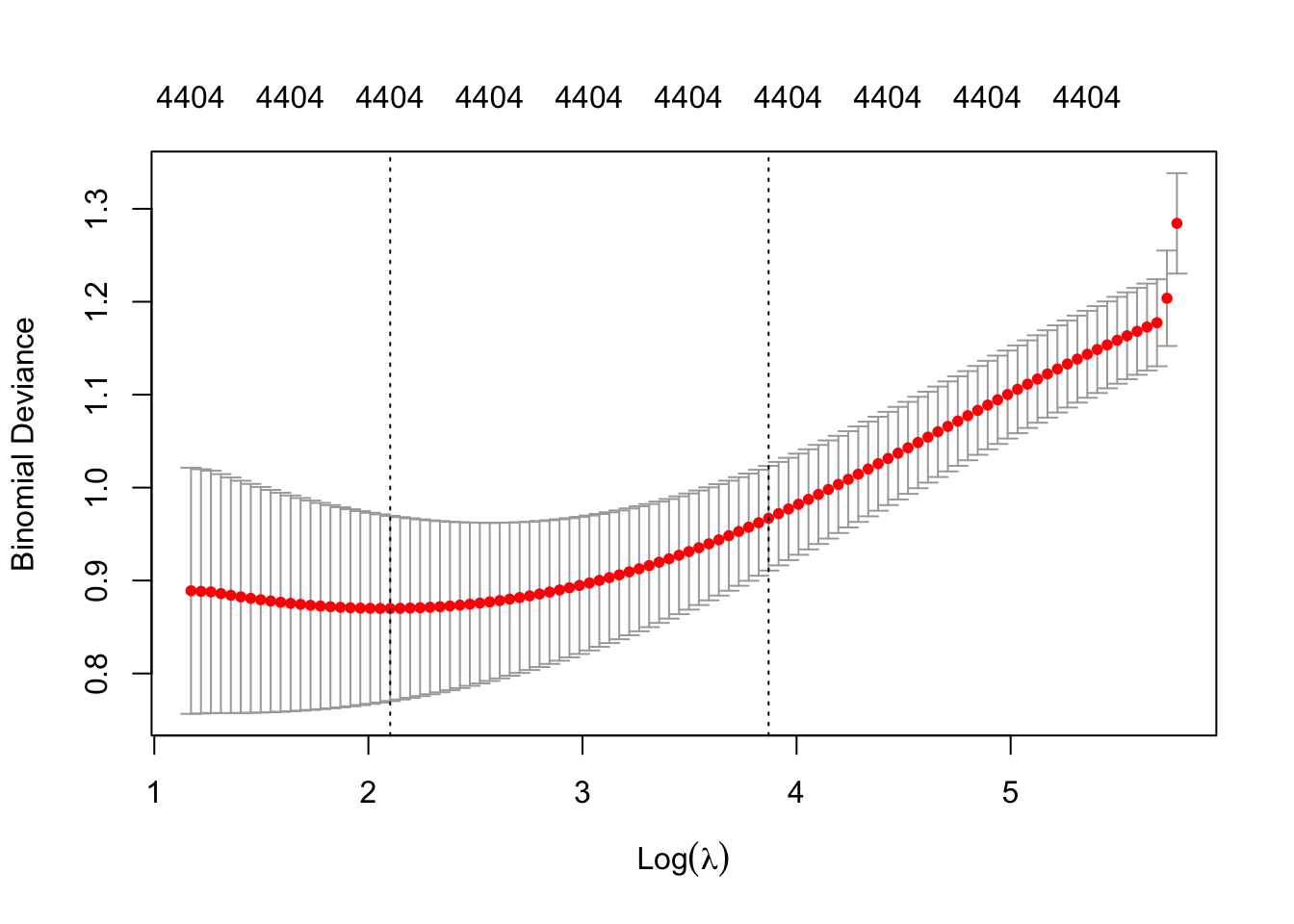
cv_ridge <- cv.glmnet(X, y, family = "binomial", alpha = 0, type.measure = "class")
plot(cv_ridge)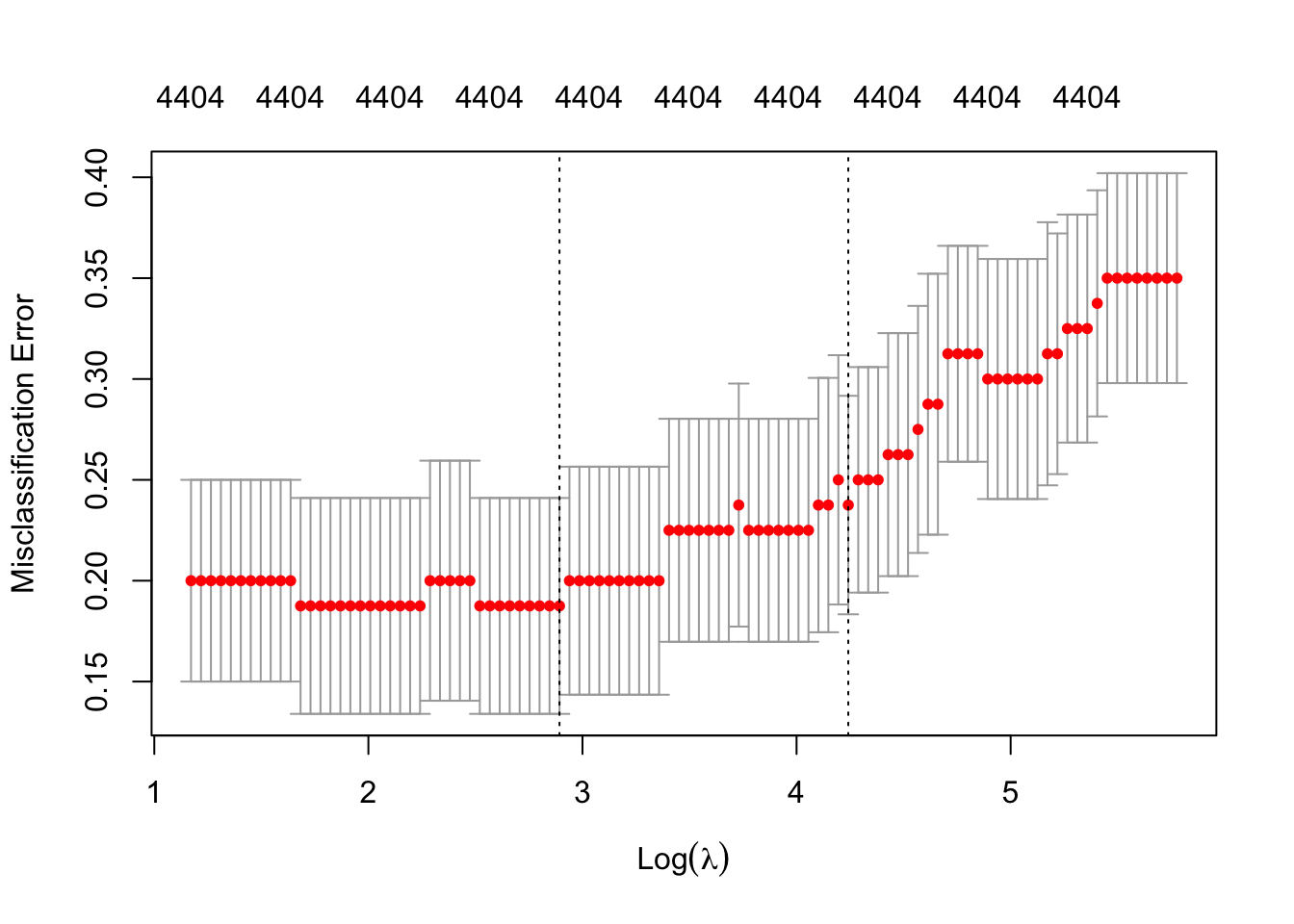
lasso_model <- glmnet(X, y, family = "binomial", alpha = 1)
plot(lasso_model, xvar="lambda")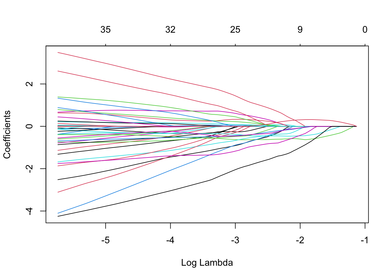
cv_lasso <- cv.glmnet(X, y, family = "binomial", alpha = 1)
plot(cv_lasso)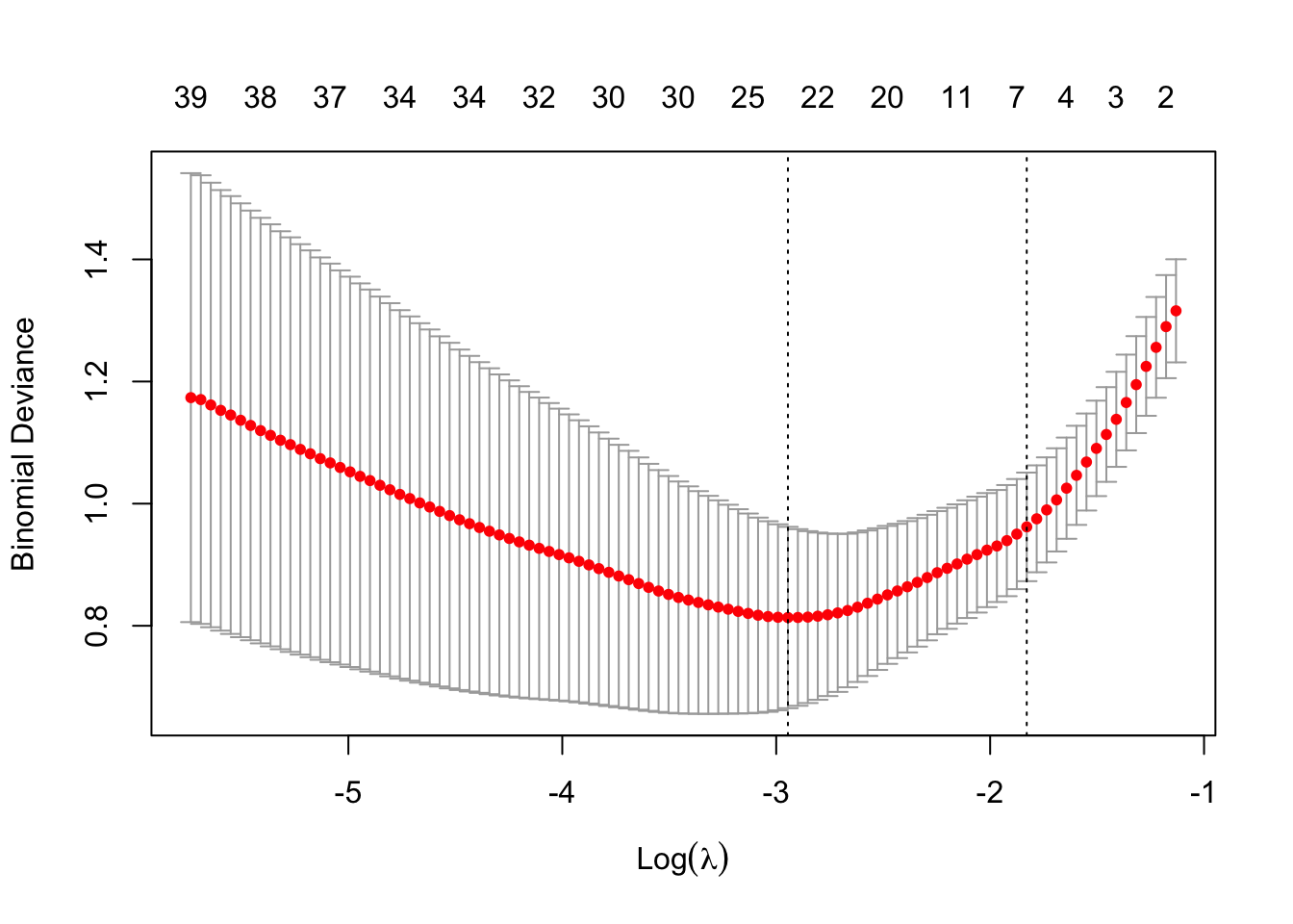
cv_lasso <- cv.glmnet(X, y, family = "binomial", alpha = 1, type.measure = "class")
plot(cv_lasso)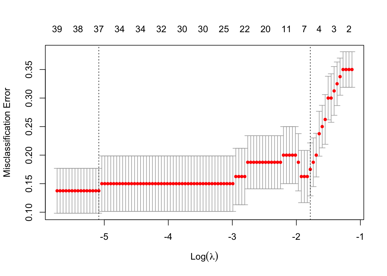
(ridge_cv_error <- min(cv_ridge$cvm))[1] 0.1875(lasso_cv_error <- min(cv_lasso$cvm))[1] 0.1375sum(coef(cv_lasso, s = "lambda.min") != 0)[1] 38sum(coef(cv_lasso, s = "lambda.1se") != 0)[1] 6if (ridge_cv_error < lasso_cv_error) {
best_model <- cv_ridge
model_type <- "ridge"
} else {
best_model <- cv_lasso
model_type <- "lasso"
}
print(paste("Selected model type:", model_type))[1] "Selected model type: lasso"y_pred <- predict(best_model, X_test, type = "response", s = "lambda.min") > 0.5
test_accuracy <- mean(y_test == y_pred)
print(paste("Test set error rate of the selected model:", round(1-test_accuracy,4)))[1] "Test set error rate of the selected model: 0.1579"Ridge regression: minimise MSE subject to \sum_{j=1}^n \beta_j^2 \leq s Lasso regression: minimise MSE subject to \sum_{j=1}^n |\beta_j| \leq s
Lasso leads to a pointier solution space: more likely to set parameters to zero.
So when should you use elastic net regression, or ridge, lasso, or plain linear regression (i.e., without any regularization)? It is almost always preferable to have at least a little bit of regularization, so generally you should avoid plain linear regression. Ridge is a good default, but if you suspect that only a few features are useful, you should prefer lasso or elastic net because they tend to reduce the useless features’ weights down to zero, as discussed earlier. In general, elastic net is preferred over lasso because lasso may behave erratically when the number of features is greater than the number of training instances or when several features are strongly correlated.