Lab 2: Simple Linear Regression

Questions

Conceptual Questions

1. Solution Prove that, in simple linear regression, the Least Squares coefficient estimates (LSE) for $\widehat{\beta}_0$ and $\widehat{\beta}_1$ are:

   $\widehat{\beta}_0 = \overline{y} - \widehat{\beta}_1 \overline{x}$

   $\widehat{\beta}_1 = \frac{\sum_{i=1}^{n} (x_i-\overline{x}) \cdot (y_i-\overline{y})}{\sum_{i=1}^{n} (x_i-\overline{x})^2} = \frac{S_{xy}}{S_{xx}}$

2. Solution Forensic scientists use various methods for determining the likely time of death from post-mortem examination of human bodies. A recently suggested objective method uses the concentration of a compound (3-methoxytyramine or 3-MT) in a particular part of the brain. In a study of the relationship between post-mortem interval and the concentration of 3-MT, samples of the approximate part of the brain were taken from coroners cases for which the time of death had been determined form eye-witness accounts. The intervals ($x$; in hours) and concentrations ($y$; in parts per million) for 18 individuals who were found to have died from organic heart disease are given in the following table. For the last two individuals (numbered 17 and 18 in the table) there was no eye-witness testimony directly available, and the time of death was established on the basis of other evidence including knowledge of the individuals’ activities.

   Observation number	Interval ($x$)	Concentration ($y$)
   1	5.5	3.26
   2	6.0	2.67
   3	6.5	2.82
   4	7.0	2.80
   5	8.0	3.29
   6	12.0	2.28
   7	12.0	2.34
   8	14.0	2.18
   9	15.0	1.97
   10	15.5	2.56
   11	17.5	2.09
   12	17.5	2.69
   13	20.0	2.56
   14	21.0	3.17
   15	25.5	2.18
   16	26.0	1.94
   17	48.0	1.57
   18	60.0	0.61

   $\sum x =337$, $\sum x^2 = 9854.5$, $\sum y = 42.98$, $\sum y^2 = 109.7936$, $\sum x y = 672.8$

   In this investigation you are required to explore the relationship between concentration (regarded the responds/dependent variable) and interval (regard as the explanatory/independent variable).

   1. Construct a scatterplot of the data. Comment on any interesting features of the data and discuss briefly whether linear regression is appropriate to model the relationship between concentration of 3-MT and the interval from death.

   2. Calculate the correlation coefficient $R$ of the data, and use it to test the null hypothesis that the population correlation coefficient $\rho$ is equal to zero. For this task, you may use the fact that, under the strong assumptions, if $H_0: \rho=0$ is true, then $$R \frac{\sqrt{n-2}}{\sqrt{1-R^2}} \sim t_{n-2}.$$

   3. Calculate the equation of the least-squares fitted regression line and use it to estimate the concentration of 3-MT:

      1. after 1 day and

      2. after 2 days.

      Comment briefly on the reliability of these estimates.

   4. A shortcut formula for the unbiased estimate of $\sigma^2$ (variance of the errors in linear regression) is given in the “Orange Formulae Book” (p.24) as $$s^2=\hat{\sigma}^2=\frac{1}{n-2}\left(S_{yy}-\frac{S_{xy}^2}{S_{xx}}\right).$$ Use this formula to compute $s^2$ for the data in this question.

   5. Calculate a 99% confidence interval for the slope of the regression line. Using this confidence interval, test the hypothesis that the slope of the regression line is equal to zero. Comment on your answer in relation to the answer given in part (2) above.

3. $\star$ Solution A university wishes to analyse the performance of its students on a particular degree course. It records the scores obtained by a sample of 12 students at the entry to the course, and the scores obtained in their final examinations by the same students. The results are as follows:

   Student	A	B	C	D	E	F	G	H	I	J	K	L
   Entrance exam score $x$ (%)	86	53	71	60	62	79	66	84	90	55	58	72
   Final paper score $y$ (%)	75	60	74	68	70	75	78	90	85	60	62	70

   $\sum x = 836$, $\sum y = 867$, $\sum x^2 = 60,\!016$, $\sum y^2 = 63,\!603$, $\sum (x-\overline{x})(y-\overline{y}) = 1,\!122$.

   1. Calculate the fitted linear regression equation of $y$ on $x$.

   2. Under the strong assumptions, it can be shown that $$\frac{s^2}{\sigma^2/(n-2)} \sim \chi^2_{n-2},$$ where $s^2$ is the unbiased estimate of $\sigma^2$ in simple linear regression. Knowing this, calculate an estimate of the variance $\sigma^2$ and obtain a 90% confidence interval for $\sigma^2$, for the above data.

   3. By considering the slope parameter, formally test whether the data is positively correlated.

   4. Calculate the proportion of variance explained by the model. Hence, comment on the fit of the model.

4. Solution Complete the following ANOVA table for a simple linear regression with $n=60$ observations:

   Source	D.F.	Sum of Squares	Mean Squares	F-Ratio
   Regression	____	____	____	____
   Error	____	____	8.2
   Total	____	639.5

5. $\star$ Solution Consider a fitted simple linear regression model (via least squares) with estimated parameters $\widehat{\beta}_0$ and $\widehat{\beta}_1$. Let $x_0$ be a new (but known) observation (i.e., not in the training set used to estimate the parameters). Your prediction of the response for $x_0$ would be $\widehat{y}_0 = \widehat{\beta}_0 + \widehat{\beta}_1 x_0$.

   1. Show that the variance of this prediction is $$\mathbb{V}(\widehat{y}_0 | \boldsymbol{x} ) = \left( \dfrac{1}{n}+\frac{\left( \overline{x}-x_{0}\right) ^{2}}{S_{xx}}\right) \sigma ^{2}.$$ Note you may use as given the expressions for the (co)-variances of $\widehat{\beta}_0, \widehat{\beta}_1$ given in the lecture.
   2. Notice how $\widehat{y}_0 = \widehat{\beta}_0 + \widehat{\beta}_1 x_0$ does not contain an “error term” (because the only reasonable prediction of the error term is $0$). But this means that the variance of $\widehat{y}_0$ computed above should be viewed as the variance of the “predicted mean” of the new observation $Y_0$. What is the variance of the predicted individual response $\widehat{Y}_0$? Hint: $\widehat{Y}_0=\widehat{\beta}_0 + \widehat{\beta}_1 x_0 + \epsilon_0$.

6. $\star$ Solution Suppose you are interested in relating the accounting variable EPS (earnings per share) to the market variable STKPRICE (stock price). Then, a regression equation was fitted using STKPRICE as the response variable with EPS as the predictor variable. Following is the computer output from your fitted regression. You are also given that: $\overline{x}=2.338$, $\overline{y}=40.21$, $s_{x}=2.004$, and $s_{y}=21.56.$ (Note that: $s_x^2=\frac{S_{xx}}{n-1}$ and $s_y^2=\frac{S_{yy}}{n-1}$)

    Regression Analysis                                                                  
    The regression equation is                                                           
    STKPRICE = 25.044 + 7.445 EPS                                                        
   
    Predictor                       Coef     SE Coef   T       p                 
    Constant                        25.044   3.326     7.53    0.000             
    EPS                             7.445    1.144     6.51    0.000             
   
    Analysis of Variance                                                                 
    SOURCE                          DF       SS        MS      F       p       
    Regression                      1        10475     10475   42.35   0.000   
    Error                           46       11377     247                         
    Total                           47       21851                                   

   1. Compute $s$ and $R^{2}$.

   2. Calculate the correlation coefficient of EPS and STKPRICE.

   3. Estimate the STKPRICE given an EPS of $2. Provide 95% confidence intervals on both the “predicted mean” and the “predicted individual response” for STKPRICE (these are defined in an previous question ). You may assume that the predicted mean and predicted response are approximately Normal (this is not exactly true, even under the strong assumptions, but a reasonable assumption if the sample size $n$ is decently large). Comment on the difference between those two confidence intervals.

   4. Provide a 95% confidence interval for the slope coefficient $\beta$.

   5. Describe how you would check if the errors have constant variance.

   6. Perform a test of the significance of EPS in predicting STKPRICE at a level of significance of 5%.

   7. Test the hypothesis $H_{0}:\beta =6$ against $H_{a}:\beta >6$ at a level of significance of 5%.

7. Solution (Modified Institute Exam Question) As part of an investigation into health service funding a working party was concerned with the issue of whether mortality could be used to predict sickness rates. Data on standardised mortality rates and standardised sickness rates were collected for a sample of 10 regions and are shown in the table below:

   Region	Mortality rate $m$ (per 100,000)	Sickness rate $s$ (per 100,000)
   1	125.2	206.8
   2	119.3	213.8
   3	125.3	197.2
   4	111.7	200.6
   5	117.3	189.1
   6	100.7	183.6
   7	108.8	181.2
   8	102.0	168.2
   9	104.7	165.2
   10	121.1	228.5

   Data summaries: $\sum m=1136.1$, $\sum m^2=129,853.03$, $\sum s=1934.2$, $\sum s^2=377,700.62$, and $\sum ms=221,022.58$.

   1. Calculate the correlation coefficient between the mortality rates and the sickness rates. Conduct a statistical test on whether the underlying population correlation coefficient is zero against the alternative that it is positive. Hint: use the test statistic provided in this previous question.

   2. Noting the issue under investigation, draw an appropriate scatterplot for these data and comment on the relationship between the two rates.

   3. Determine the fitted linear regression of sickness rate on mortality rate. Then, test whether the underlaying slope coefficient can be considered to be larger than 2.0.

   4. For a region with mortality rate 115.0, estimate the expected sickness rate.

More Proofs

8. Solution Prove that the LSE of $\beta_0$ and $\beta_1$ are unbiased.

9. Solution Prove that the MLE estimates of $\beta_0$ and $\beta_1$ are equal to the ones given by LSE.

10. Solution Prove that TSS=RSS+MSS.

11. Solution Express MSS in terms of a) $\hat{\beta}_1$ and b) $\hat{\beta}_1^2$.

12. Solution Prove the following variance formulas:

    $$\begin{align*} \mathbb{V}\left( \widehat{\beta}_0 |X\right) &= \sigma^2\left(\frac{1}{n}+\frac{\overline{x}^2}{S_{xx}}\right)\\ \mathbb{V}\left( \widehat{\beta}_1 |X\right) &= \frac{\sigma^2}{S_{xx}} \\ \text{Cov}\left( \widehat{\beta}_0, \widehat{\beta}_1 | X\right) &= -\frac{ \overline{x} \sigma^2}{S_{xx}} \end{align*}$$

Applied Questions

1. Solution $\star$ (ISLR2, Q3.8) This question involves the use of simple linear regression on the Auto data set.

   1. Use the lm() function to perform a simple linear regression with mpg as the response and horsepower as the predictor. Use the summary() function to print the results. Comment on the output.
      For example:

      1. Is there a relationship between the predictor and the response?

      2. How strong is the relationship between the predictor and the response?

      3. Is the relationship between the predictor and the response positive or negative?

      4. What is the predicted mpg associated with a horsepower of 98? What are the associated 95% confidence and prediction intervals?

   2. Plot the response and the predictor. Use the abline() function to display the least squares regression line.

   3. Use the plot() function to produce diagnostic plots of the least squares regression fit. Comment on any problems you see with the fit.

2. Solution (ISLR2, Q3.11) In this problem we will investigate the $t$-statistic for the null hypothesis $H_0:\beta = 0$ in simple linear regression without an intercept. To begin, we generate a predictor $x$ and a response $y$ as follows.

   set.seed(1)
   x <- rnorm(100)
   y <- 2 * x + rnorm(100)

   1. Perform a simple linear regression of $y$ onto $x$, without an intercept. Report the coefficient estimate $\widehat{\beta}$, the standard error of this coefficient estimate, and the $t$-statistic and $p$-value associated with the null hypothesis $H_0:\beta = 0$. Comment on these results. (You can perform regression without an intercept using the command lm(y ~ x+0).)

   2. Now perform a simple linear regression of $x$ onto $y$ without an intercept, and report the coefficient estimate, its standard error, and the corresponding $t$-statistic and $p$-values associated with the null hypothesis $H_0:\beta = 0$. Comment on these results.

   3. What is the relationship between the results obtained in (a) and (b)?

   4. For the regression of $Y$ onto $X$ without an intercept, the $t$-statistic for $H_0:\beta = 0$ takes the form $\widehat{\beta}/\text{SE}(\widehat{\beta})$, where $\widehat{\beta}$ is given by (3.38), and where $$\text{SE}(\widehat{\beta}) = \sqrt{\frac{\sum_{i}^n(y_i - x_i\widehat{\beta})^2}{(n-1)\sum_{i'=1}^nx_{i'}^2}}$$ (These formulas are slightly different from those given in Sections 3.1.1 and 3.1.2, since here we are performing regression without an intercept.) Show algebraically, and confirm numerically in R, that the t-statistic can be written as $$\frac{(\sqrt{n-1})\sum_{i=1}^nx_i y_i}{\sqrt{(\sum_{i=1}^nx_i^2)(\sum_{i'=1}^n y_{i'}^2) - (\sum_{i'=1}^n x_{i'}y_{i'})^2}}$$

   5. Using the results from (d), argue that the $t$-statistic for the regression of $y$ onto $x$ is the same as the $t$-statistic for the regression of $x$ onto $y$.

   6. In R, show that when regression is performed with an intercept, the $t$-statistic for $H_0: \beta_1 = 0$ is the same for the regression of $y$ onto $x$ as it is for the regression of $x$ onto $y$.

Solutions

Conceptual Questions

1. Question We determine $\widehat{\beta}_0$ and $\widehat{\beta}_1$ by minimizing the error. Hence, we use least squares estimates (LSE) for $\widehat{\beta}_0$ and $\widehat{\beta}_1$: $$\underset{\beta_0,\beta_1}{\min}\left\{S\left( \widehat{\beta}_0, \widehat{\beta}_1 \right)\right\}=\underset{\beta_0,\beta_1}{\min}\left\{\sum_{i=1}^{n}\left( y_{i}-\left(\widehat{\beta}_0 + \widehat{\beta}_1 x_{i}\right) \right)^{2}\right\}.$$ The minimum is obtained by setting the first order condition (FOC) to zero: $$\begin{aligned} \frac{\partial S\left( \widehat{\beta}_0,\widehat{\beta}_1\right)}{\partial \widehat{\beta}_0}&=-2\sum_{i=1}^{n} y_{i}-\left(\widehat{\beta}_0+\widehat{\beta}_1x_{i}\right)\\ \frac{\partial S\left( \widehat{\beta}_0,\widehat{\beta}_1\right)}{\partial \widehat{\beta}_1}&=-2\sum_{i=1}^{n}x_{i}\left(y_{i}-\left( \widehat{\beta}_0+\widehat{\beta}_1x_{i}\right) \right). \end{aligned}$$

   The LSE $\widehat{\beta}_0$ and $\widehat{\beta}_1$ are given by setting the FOC equal to zero: $$\begin{aligned} \sum_{i=1}^{n}y_{i} =& n\widehat{\beta}_{0}+\widehat{\beta}_{1}\sum_{i=1}^{n}x_{i}\\ \sum_{i=1}^{n}x_{i}y_{i} =& \widehat{\beta}_{0}\sum_{i=1}^{n}x_{i}+\widehat{ \beta }_{1}\sum_{i=1}^{n}x_{i}^{2}. \end{aligned}$$

   So we have

   $$\begin{aligned} \widehat{\beta}_{0}=& \frac{\sum_{i=1}^{n}y_i-\widehat{\beta}_{1} \sum_{i=1}^{n}x_i}{n}=\overline{y} - \widehat{\beta}_1\overline{x}, \text{ and} \\ \widehat{\beta}_{1}=& \frac{\sum_{i=1}^{n}x_iy_i-\widehat{\beta}_{0} \sum_{i=1}^{n}x_i}{\sum_{i=1}^{n}x^2_i} \,. \end{aligned}$$

   Next step: Rearranging so that $\widehat{\beta}_0$ and $\widehat{\beta}_1$ become functions of $\sum_{i=1}^ny_i$, $\sum_{i=1}^nx_i$, $\sum_{i=1}^nx^2_i$, and $\sum_{i=1}^nx_iy_i$

   $$\begin{aligned} \widehat{\beta}_{0}=& \frac{\sum_{i=1}^{n}y_i-\left(\frac{\sum_{i=1}^{n}x_iy_i-\widehat{\beta}_{0} \sum_{i=1}^{n}x_i}{\sum_{i=1}^{n}x^2_i}\right) \sum_{i=1}^{n}x_i}{n}\\ \hskip-10mm\left(1-\frac{\left(\sum_{i=1}^{n}x_i\right)^2}{n\sum_{i=1}^{n}x^2_i}\right)\widehat{\beta}_{0}=&\frac{\sum_{i=1}^{n}x^2_i\sum_{i=1}^{n}y_i-\left(\sum_{i=1}^{n}x_iy_i\right) \sum_{i=1}^{n}x_i}{n\sum_{i=1}^{n}x^2_i}\\ \widehat{\beta}_{0}\overset{*}{=}& \frac{\sum_{i=1}^{n}y_i\left(\sum_{i=1}^{n}x_i^2\right)-\sum_{i=1}^{n}x_iy_i\sum_{i=1}^{n}x_i}{n\sum_{i=1}^{n}x^2_i -\left(\sum_{i=1}^{n}x_i\right)^2}. \end{aligned}$$

   *$(1-a/b)c = d/b \rightarrow (bc-ac)/b=d/b \rightarrow c=d/(b-a)$.

   And $\widehat{\beta}_0$’s in line (6) was subbed into $\widehat{\beta}_1$ in line (7). At this point, $\widehat{\beta}_0$ is done. So we’ll continue with $\widehat{\beta}_1$.

   From the previous steps we have: $$\begin{aligned} \widehat{\beta}_{0}=& \frac{\sum_{i=1}^{n}y_i-\widehat{\beta}_{1} \sum_{i=1}^{n}x_i}{n}\\ \widehat{\beta}_{1}=& \frac{\sum_{i=1}^{n}x_iy_i-\widehat{\beta}_{0} \sum_{i=1}^{n}x_i}{\sum_{i=1}^{n}x^2_i}. \end{aligned}$$ thus: $$\begin{aligned} \widehat{\beta}_{1}=& \frac{n\sum_{i=1}^{n}x_iy_i-\left(\sum_{i=1}^{n}y_i-\widehat{\beta}_{1} \sum_{i=1}^{n}x_i\right)\sum_{i=1}^{n}x_i}{n\sum_{i=1}^{n}x^2_i}\\ \left(1-\frac{\left(\sum_{i=1}^nx_i\right)^2}{n\sum_{i=1}^{n}x_i^2}\right)\widehat{\beta}_{1}=& \frac{n\sum_{i=1}^{n}x_iy_i-\sum_{i=1}^{n}y_i\sum_{i=1}^{n}x_i}{n\sum_{i=1}^{n}x^2_i}\\ \widehat{\beta}_{1}\overset{*}{=}& \frac{n\sum_{i=1}^{n}x_iy_i-\sum_{i=1}^{n}y_i\sum_{i=1}^{n}x_i}{n\sum_{i=1}^{n}x^2_i-\left(\sum_{i=1}^{n}x_i\right)^2}. \end{aligned}$$

   *$(1-a/b)c = d/b \rightarrow (bc-ac)/b=d/b \rightarrow c=d/(b-a)$.

   Using the notations, we have an easier way to write $\widehat{\beta}_{1}$: $$\begin{aligned} \widehat{\beta}_{1}=& \frac{n\sum_{i=1}^{n}x_iy_i-\sum_{i=1}^{n}y_i\sum_{i=1}^{n}x_i}{n\sum_{i=1}^{n}x^2_i-\left(\sum_{i=1}^{n}x_i\right)^2} \\%= \frac{nS_{xy}-S_xS_y}{nS_{xx}-S^2_x}\\ =&\frac{n\left(\sum_{i=1}^{n}x_iy_i-\sum_{i=1}^{n}y_i\sum_{i=1}^{n}x_i\cdot\frac{n}{n^2}\right)}{n\left(\sum_{i=1}^{n}x^2_i-\left(\sum_{i=1}^{n}x_i\right)^2\cdot\frac{n}{n^2}\right)}\\ =&\frac{\sum_{i=1}^{n}x_iy_i-n\overline{x} \,\overline{y}}{\sum_{i=1}^{n}x^2_i-n\overline{x}^2}\\ \overset{*}{=}&\frac{\sum_{i=1}^{n}x_iy_i- \sum_{i=1}^{n}x_i\overline{y} -\sum_{i=1}^{n}y_i\overline{x} +n \overline{x}\,\overline{y}}{\sum_{i=1}^{n}x^2_i+\sum_{i=1}^{n}\overline{x}^2-2\sum_{i=1}^{n}x_i\overline{x}}\\ =&\frac{\sum_{i=1}^{n}(x_i-\overline{x})\cdot(y_i-\overline{y})}{\sum_{i=1}^{n}(x_i-\overline{x})^2} =\frac{S_{xy}}{S_{xx}} \,. \end{aligned}$$

   *$\sum_{i=1}^{n}x_i\overline{y}=\sum_{i=1}^{n}x_i\frac{\sum_{i=1}^{n}y_i}{n}=\sum_{i=1}^{n}y_i\frac{\sum_{i=1}^{n}x_i}{n}=\sum_{i=1}^{n}y_i\overline{x}=n\frac{\sum_{i=1}^{n}x_i}{n}\frac{\sum_{i=1}^{n}y_i}{n}=n\overline{x}\overline{y}$.

2. Question

   1. 

      Scatterplot of concentration against interval.

      Interesting features are that, in general, the concentration of 3-MT in the brain seems to decrease as the post mortem interval increases. Another interesting feature is that we observe two observations with a much higher post mortem interval than the other observations.
      The data seems to be appropriate for linear regression. The linear relationship seems to hold,especially for values of interval between 5 and 26 (we have enough observations for that). Care should be taken into account when evaluating $y$ for $x$ lower than 5 and larger than 26 (only two observations) because we do not know whether the linear relationship between $x$ and $y$ still holds then.

   2. We test: $$H_0: \rho=0 \hskip3mm \text{v.s.} \hskip3mm H_1: \rho\neq0$$ The corresponding test statistic is given by:

      $$T=\frac{R\sqrt{n-2}}{\sqrt{1-R^2}} \sim t_{n-2}.$$ We reject the null hypothesis for large and small values of the test statistic.
      We have $n=18$ and the correlation coefficient is given by: $$\begin{aligned} r =& \frac{\sum x_i\cdot y_i - n \overline{x}\overline{y} }{ \sqrt{(\sum x_i^2 - n\overline{x}^2) (\sum y_i^2 - n\overline{y}^2)} }\\ =& \frac{672.8 - 18\cdot337/18\cdot42.98/18}{\sqrt{(9854.5-337^2/18)\cdot(109.7936-42.98^2/18)} } = -0.827 \end{aligned}$$ Thus, the value of our test statistic is given by: $$T=\frac{-0.827\sqrt{16}}{\sqrt{1-(-0.827)^2}}=-5.89.$$ From Formulae and Tables page 163 we observe $\mathbb{P}(t_{16}\leq-4.015)\overset{*}{=}\mathbb{P}(t_{16}\geq4.015)=0.05\%$, * using symmetry property of the student-$t$ distribution. We observe that the value of our test statistic (-5.89) is smaller than -4.015, thus our $p$-value should be smaller than $2\cdot0.05\%=0.1\%$. Thus, we can reject the null hypothesis even at a significance level of 0.1%, hence we can conclude that there is a linear dependency between interval and concentration. Note that the alternative hypothesis is here a linear dependency and not negative linear dependency, so you do accept the alternative by rejecting the null hypothesis. Although, when you would use as alternative hypothesis negative dependency, you would accept this alternative, due to the construction of the test we have to use the phrase “a linear dependency” and not “a negative linear dependency”.

   3. The linear regression model is given by: $$y=\alpha + \beta x +\epsilon$$ The estimate of the slope is given by: $$\begin{aligned} \widehat{\beta} =& \frac{ \sum x_iy_i -n\sum x_i/n\sum y_i/n }{\sum x_i^2 -n(\sum x_i/n)^2}\\ =& \frac{ 672.8 - 337\cdot42.98/18 }{9854.4 -334^2/18} = -0.0372008 \end{aligned}$$ The estimate of the intercept is given by: $$\begin{aligned} \widehat{\alpha}=& \overline{y}-\widehat{\beta}\overline{x}\\ =& 42.98/18 + 0.0372008 \cdot337/18 = 3.084259 \end{aligned}$$ Thus, the estimate of $y$ given a value of $x$ is given by: $$\begin{aligned} \widehat{y}=&\widehat{\alpha} + \widehat{\beta} x\\ =&3.084259 - 0.0372008 x \end{aligned}$$

      1. One day equals 24 hours, i.e., $x=24$, thus $\widehat{y}=\widehat{\alpha} + \widehat{\beta}24=3.084259 - 0.0372008 \cdot 24 = 2.19$

      2. Two day equals 48 hours, i.e., $x=48$, thus $\widehat{y}=\widehat{\alpha} + \widehat{\beta}24=3.084259 - 0.0372008 \cdot 48 = 1.30$

      The data set contains accurate data up to 26 hours, as for observations 17 and 18 (at 48 hour and 60 hours respectively) there was no eye-witness testimony direct available. Predicting 3-MT concentration after 26 hours may not be advisable, even though $x=48$ is within the range of the $x$-values (5.5 hours to 60 hours).

   4. We calculate $$\begin{aligned} \widehat{\sigma}^2 &= \frac{1}{n-2}\left(\sum y^2_i- (\sum y_i)^2/n - \frac{(\sum x_iy_i - \sum x_i\sum y_i/n)^2}{\sum x_i^2 - (\sum x_i)^2/n}\right) \\ &= \frac{1}{16}\left(109.7936- 42.98^2/18 - \frac{(672.8 - 337\cdot42.98/18)^2}{9854.5 - 337^2/18}\right) = 0.1413014 , \end{aligned}$$

   5. The pivotal quantity is given by: $$\frac{\beta-\widehat{\beta}}{\text{SE}(\widehat{\beta})} \sim t_{n-2}.$$ The standard error is $$\text{SE}(\widehat{\beta}) = \sqrt{\frac{\widehat{\sigma}^2}{\sum x_i^2 - n\overline{x}^2}} = \sqrt{\frac{0.1413014 }{9854.5 - 337^2/18}} = 0.00631331.$$ From Formulae and Tables page 163 we have $t_{16,1-0.005} = 2.921$. Using the test statistic, the 99% confidence interval of the slope is given by: $$\begin{aligned} \widehat{\beta}-t_{16,1-\alpha/2}\text{SE}(\widehat{\beta})<&\beta<\widehat{\beta}+t_{16,1-\alpha/2}\text{SE}(\widehat{\beta})\\ - 0.0372008 -2.921\cdot 0.00631331<&\beta<- 0.0372008 +2.921\cdot 0.00631331\\ -0.055641979<&\beta<-0.0188 . \end{aligned}$$ Thus the 99% confidence interval of $\beta$ is given by: $(-0.055641979, -0.0188)$. Note that $\beta=0$ in not within the 99% confidence interval, therefore we would reject the null hypothesis that $\beta$ equals zero and accept the alternative that $\beta\neq0$ at a 1% level of significance. This confirms the result in (2) where the correlation coefficient was shown to not equal zero at the 1% significance level.

3. $\star$ Question

   1. The linear regression model is given by: $$y_i =\alpha + \beta x_i +\epsilon_i,$$ where $\epsilon_i \sim N(0,\sigma^2)$ i.i.d. distributed for $i=1,\ldots,n$.
      The fitted linear regression equation is given by:

      $$\widehat{y} = \widehat{\alpha} + \widehat{\beta}x.$$ The estimated coefficients of the linear regression model are given by (see Formulae and Tables p.24): $$\begin{aligned} \widehat{\beta} &= \frac{s_{xy}}{s_{xx}} = \frac{1122}{\sum_{i=1}^n x_i^2 -n \overline{x}^2} \\ &= \frac{1122}{60016 - 12 \cdot \left(\frac{836}{12}\right)^2} = \frac{1122}{1774.67} = 0.63223 \\ \widehat{\alpha} &= \overline{y} - \widehat{\beta} \overline{x} = \frac{\sum_{i=1}^n y_i}{n} - \widehat{\beta}\frac{\sum_{i=1}^n x_i}{n} \\ &= \frac{867}{12} - 0.63223\cdot \frac{836}{12} = 28.205. \end{aligned}$$ Thus, the fitted linear regression equation is given by: $$\widehat{y} = 28.205 + 0.63223\cdot x.$$

   2. We have $$s^2=\hat{\sigma}^2=\frac{1}{n-2}\left(S_{yy}-\frac{S_{xy}^2}{S_{xx}}\right)$$ From the previous part, we already have $S_{xx}=1774.67$, so $$s^2= \frac{1}{10} \cdot \left(63603-(867^2/12) -1122^2/1774.67 \right) = 25.289$$

      Then, we know the pivotal quantity: $$\frac{s^2}{\sigma^2/(n-2)} \sim \chi^2_{n-2} \,.$$ Note: we have $n-2$ degrees of freedom because we have to estimate two parameters form the data ($\widehat{\alpha}$ and $\widehat{\beta}$). Calling $\chi^2_{\alpha,\nu}$ the $\alpha$-quantile of a $\chi^2$ with $\nu$ degrees of freedom, we have $$\begin{align*} &\mathbb{P}\left[\chi^2_{0.05,10} < \frac{s^2}{\sigma^2/(n-2)} < \chi^2_{0.95,10} \right] = 0.9\\ &\mathbb{P}\left[\frac{1}{\chi^2_{0.05,10}} > \frac{\sigma^2/(n-2)}{s^2} > \frac{1}{\chi^2_{0.95,10}} \right] = 0.9 \end{align*}$$

      Thus, we have that the 90% confidence interval is given by: $$\begin{aligned} \frac{10 s^2}{\chi^2_{0.95,10}} &< \sigma^2 < \frac{10 s^2}{\chi^2_{0.05,10}} \\ \frac{10\cdot 25.289}{18.3} &< \sigma^2 < \frac{10\cdot 25.289}{3.94} \\ 13.8 &< \sigma^2 < 64.2 \end{aligned}$$ Finally, for our data the 90% confidence interval of $\sigma^2$ is given by $(13.8, 64.2)$.

   3. 1. We test the following: $$H_0:\beta=0 \hskip3mm \text{v.s.} \hskip3mm H_1:\beta> 0,$$ with a level of significance $\alpha=0.05$.
         
      2. The test statistic is: $$T = \frac{\widehat{\beta}-\beta}{\sqrt{\widehat{\sigma^2}/\left(\sum_{i=1}^n (x_i-\overline{x})^2\right) }} \sim t_{n-2}$$
      3. The rejection region of the test is given by: $$C= \{(X_1,\ldots,X_n): T\in(t_{10,1-0.05},\infty) \} = \{(X_1,\ldots,X_n): T\in(1.812,\infty) \}$$
      4. The value of the test statistic is given by: $$T = \frac{0.63223-0}{\sqrt{25.289/(\sum_{i=1}^nx^2_i-n\overline{x}^2) }} =\frac{0.63223-0}{\sqrt{25.289/(60016-836^2/12 )}} = 5.296.$$
      5. The value of the test statistic is in the rejection region, hence we reject the null hypothesis of a zero correlation.

   4. The proportion of the variability explained by the model is given by: $$\begin{aligned} R^2 =& \frac{\text{MSS}}{\text{TSS}} = 1-\frac{\text{RSS}}{\text{TSS}}\\ =& 1 - \frac{(n-2)s^2}{S_{yy}}\\ =& 1 - (10 \cdot 25.289)/(63603 - (867^2/12))\\ =& 0.7372. \end{aligned}$$ Hence, a fairly large proportion of the variability of $Y$ is explained by $X$.

4. Question The completed ANOVA table is given below:

   Source	D.F.	Sum of Squares	Mean Squares	F-Ratio
   Regression	$1$	$639.5-475.6=163.9$	$163.9$	$\frac{163.9}{8.2}=19.99$
   Error	$58$	$8.2 \times 58=475.6$	$8.2$
   Total	$59$	$639.5$

5. Question

   1. We have that $$\begin{aligned} \mathbb{V}\left( \widehat{y}_{0} | \boldsymbol{x} \right) &= \mathbb{V}\left( \widehat{\beta}_0+\widehat{\beta}_1x_{0} | \boldsymbol{x} \right) \\ &= \mathbb{V}\left( \widehat{\beta}_0 | \boldsymbol{x} \right) +x_{0}^{2}\mathbb{V}\left( \widehat{\beta}_1 | \boldsymbol{x} \right) +2x_{0}\text{Cov}\left( \widehat{\beta}_0,\widehat{\beta}_1 | \boldsymbol{x} \right) \\ &= \left( \dfrac{1}{n}+\frac{\overline{x}^{2}}{S_{xx}}\right) \sigma ^{2}+x_{0}^{2}\frac{\sigma ^{2}}{S_{xx}}+2x_{0}\left( \frac{-\overline{x}\sigma ^{2}}{S_{xx}}\right) \\ &= \left( \dfrac{1}{n}+\frac{\overline{x}^{2}-2x_{0}\overline{x}+x_{0}^{2}}{S_{xx}}\right) \sigma ^{2} \\ &= \left( \dfrac{1}{n}+\frac{\left( \overline{x}-x_{0}\right) ^{2}}{S_{xx}}\right) \sigma ^{2}. \end{aligned}$$

   2. We have $$\begin{aligned} \mathbb{V}\left(\widehat{Y}_0 | \boldsymbol{x} \right) &= \mathbb{V}\left(\widehat{y}_0 + \epsilon_0| \boldsymbol{x} \right)\\ &\overset{**}{=} \mathbb{V}\left(\widehat{y}_0 | \boldsymbol{x} \right) + \mathbb{V}\left(\epsilon_0| \boldsymbol{x} \right)\\ &=\sigma^2\left({1\over n}+{(\overline{x} - x_0)^2\over S_{xx}}\right) + \sigma^2\\ &= \sigma^2\left(1+{1\over n}+{(\overline{x} - x_0)^2\over S_{xx}}\right). \end{aligned}$$

   ** note that $\widehat{y}_0$ and $\epsilon_0$ are not correlated, because $\epsilon_0$ is the error of a new observation (which is independent of the training observations, hence independent of $\widehat{y}_0 = \widehat{\beta}_0+\widehat{\beta}_1 x_0$).

6. Question problem:

   1. We have $s^2$=RSS/$(n-2)$, hence $s=\sqrt{247}=15.716$ and $R^{2}=\frac{\text{MSS}}{\text{TSS}}=\frac{10475}{21851}=0.4794$.

   2. We know that $R^2$=MSS/TSS=$10475/21851$, and $R^{2}=r^{2}$ where $r$ is the empirical correlation. Hence, $r^{2}=0.4794\Longrightarrow r=+\sqrt{0.4794}=69.24\%$. We take the positive square root because of the positive sign of the coefficient of $EPS$.

   3. Given $EPS=2$, we have: $$\widehat{STKPRICE}=25.044+7.445\left( 2\right) =39.934.$$ Note that $s_{x}^{2}$ is the sample variance of $X$, and we have $S_{xx}=(n-1)s_x^2$. The estimated standard deviation of the predicted mean is: $$\begin{align*} s\sqrt{\left( \frac{1}{n}+\frac{\left( \overline{x}-x_{0}\right) ^{2}}{\left( n-1\right) s_{x}^{2}}\right)} & = \sqrt{247}\sqrt{\left( \frac{1}{48}+\frac{\left( 2.338-2\right) ^{2}}{\left( 47\right) \left( 2.004^{2}\right) }\right) } \\ & = 2.3012 \end{align*}$$

      Because the 97.5%-quantile of the standard Normal is $z_{0.975}=1.96$, we obtain the approximate confidance interval: $$\begin{align*} & \left( \widehat{\alpha }+\widehat{\beta}x_{0}\right) \pm z_{1-\alpha/2} \times \text{S.D.}\left( \widehat{\alpha }+\widehat{\beta}x_{0}\right) \\ & = \left( 39.934\right) \pm 1.96 \times 2.3012 \\ & = \left( 39.934\right) \pm 4.510 = \left(35.424, 44.444\right) \end{align*}$$ For the confidence interval on the “individual predicted response” $\widehat{Y}_0$, the only difference is that the estimated variance of $\widehat{Y}_0$ is larger by “$s^2$”. Hence, $$\begin{align*} \widehat{\mathbb{V}[\widehat{Y}_0]} & = 247 \times \left(1 + \frac{1}{48}+\frac{\left( 2.338-2\right) ^{2}}{\left( 47\right) \left( 2.004^{2}\right) } \right) = 253.2953 \end{align*}$$ And the confidence interval is $$\begin{align*} \widehat{y}_0 \pm \text{S.D.}[\widehat{Y}_0] & = 39.934 \pm 1.96 \sqrt{252.2953} \\ & = 39.934 \pm 31.132 = \left(8.802, 71.066 \right). \end{align*}$$ This condidence interval is much broader, which should make sense: there is far less uncertainty about the overall trend (predicted mean of $Y_0$) than about a specific data point (the actual, individual, $Y_0$).

   4. A 95% confidence interval for $\beta$ is: $$\begin{aligned} \widehat{\beta}\pm t_{1-\alpha /2,n-2}\cdot \text{SE}( \widehat{\beta} ) &= 7.445\pm 2.0147\times \frac{\sqrt{247}}{2.004\sqrt{47}} \\ &= 7.445\pm 2.305 \\ &= \left( 5.14,9.75\right) . \end{aligned}$$

   5. A scatter plot of the residuals (standardised) against either their fitted values ($\widehat{y}_i$) or their predictors ($x_i$) provides a visual tool to assess the constancy of the variation in the errors.

   6. Because the 95% confidence interval for $\beta$ computed earlier does not contain $0$, we already know that, at a level of significance of 5%, we do reject $H_0:\beta=0$. We can also double-check explicitly (it is the same price) by computing the test statistic. For the significance of the variable EPS, we test $H_{0}:\beta=0$ against $H_{a}:\beta \neq 0$. The test statistic is: $$t( \widehat{\beta} ) = \frac{\widehat{\beta}}{\text{SE}( \widehat{\beta} ) } = \frac{7.445}{1.144} = 6.508.$$ This is larger than $t_{1-\alpha /2,n-2}=2.0147$ and therefore we reject the null. There is evidence to support the fact that the EPS variable is a significant predictor of stock price.

   7. To test $H_{0}:\beta = 6$ against $H_{a}:\beta > 6$, the test statistic is given by: $$t( \widehat{\beta} ) = \frac{\widehat{\beta}-\beta_{0}}{\text{SE}(\widehat{\beta}) } = \frac{7.445-6}{1.144} = 1.263.$$ Thus, since this test statistic is smaller than $t_{1-\alpha,n-2}=t_{0.95,46}=1.676,$ we do not reject the null hypothesis.

7. Solution

   1. We have the estimated correlation coefficient: $$\begin{aligned} r =& \frac{s_{ms}}{\sqrt{s_{mm}\cdot s_{ss}}}\\ =& \frac{\sum ms - n\overline{ms}}{\sqrt{(\sum m^2 -n\overline{m}^2) \cdot (\sum s^2 -n\overline{s}^2) }}\\ =& \frac{221,022.58 - 1136.1\cdot1934.2/10}{\sqrt{(129,853.03 -1136.1^2/10) \cdot (377,700.62 -1934.2^2/10) }} = 0.764. \end{aligned}$$

      1. We have the hypothesis: $$H_0:\rho=0 \hskip3mm \text{v.s.} \hskip3mm H_1:\rho>0$$
      2. The test statistic is: $$T=\frac{r \sqrt{n-2}}{\sqrt{1-r^2}} \sim t_{n-2}$$
      3. The critical region is given by: $$C = \{(X_1,\ldots,X_n):T\in (t_{n-2,1-\alpha},\infty)\}$$
      4. The value of the test is: $$T=\frac{r \sqrt{n-2}}{\sqrt{1-r^2}} = \frac{0.764 \sqrt{10-2}}{\sqrt{1-0.764^2}} = 3.35$$
      5. We have $t_{8,1-0.005}=3.35$. Thus the $p$-value is 0.005 and we reject the null hypothesis of a zero correlation for any level of significance that is 0.005 (i.e., 0.5%) or more. This means we reject for typical significance levels used (1%, 5%).

   2. Given the issue of whether mortality can be used to predict sickness, we require a plot of sickness against mortality:

      

      Scatterplot of sickness and mortality.

      There seems to be an increase linear relationship such that mortality could be used to predict sickness.

   3. We have the estimates: $$\begin{aligned} \widehat{\beta} =& \frac{s_{ms}}{s_{mm}} = \frac{\sum ms - n\overline{ms}}{\sum m^2 -n\overline{m}^2}\\ =& \frac{221,022.58 - 1136.1\cdot1934.2/10}{ 129,853.03 -1136.1^2/10} = 1.6371\\ \widehat{\alpha} =& \overline{y} - \widehat{\beta}\overline{x} = \frac{1934.2}{10} - 1.6371 \frac{1136.1}{10} =7.426\\ \widehat{\sigma^2} =& \frac{1}{n-2} \sum_{i=1}^{n}(y_i-\widehat{y}_i)^2 =\frac{1}{n-2}\left(s_{ss} - \frac{s^2_{ms}}{s_{mm}}\right)\\ =&\frac{1}{8}\left((\sum s^2 -n\overline{s}^2) - \frac{(\sum ms -n\overline{ms})^2}{(\sum m^2 -n\overline{m}^2)}\right)\\ =&\frac{1}{8}\left(3587.656 - \frac{(1278.118)^2}{780.709}\right) =186.902\\ \mathbb{V}(\widehat{\beta}) =& \widehat{\sigma}^2/s_{mm} = 186.902/780.709 = 0.2394 \end{aligned}$$

      1. Hypothesis: $$H_0:\beta=2 \hskip3mm \text{v.s.} \hskip3mm H_1:\beta>2$$ (we set up the hypothesis this way, because then if we reject $H_0$, then we have some evidence that $\beta>2$).
      2. Test statistic: $$T=\frac{\widehat{\beta}-\beta}{\sqrt{\widehat{\sigma^2}/s_{xx}}} \sim t_{n-2}$$
      3. Critical region: $$C = \{(X_1,\ldots,X_n):T\in (t_{n-2,1-\alpha},\infty)\}$$
      4. Value of statistic: $$T=\frac{\widehat{\beta}-\beta}{\sqrt{\widehat{\sigma^2}/s_{xx}}} = \frac{1.6371-2}{\sqrt{0.2394}} = -0.74$$
      5. It is obvious we do not reject, because the test statistic is negative. Note you have from Formulae and Tables p.163 that $t_{8,95\%}=1.86$, hence a test statistic larger than that would have resulted in a rejection of $H_0$ in favour of $H_1$. Here though, we don’t have any evidence to support that $\beta>2$.

   4. For a region with $m=115$ we have the estimated value:

      $$\widehat{s} = 7.426 + 1.6371 \cdot 115 = 195.69.$$

More Proofs

8. Question For $\widehat{\beta}_0$, using the equation in line (10) in Q1:

   $$\mathbb{E} \left[ \widehat{\beta}_{0}| X\right] = \mathbb{E}\left[\frac{\sum_{i=1}^{n}y_i\left(\sum_{i=1}^{n}x_i^2\right)-\sum_{i=1}^{n}x_iy_i\sum_{i=1}^{n}x_i}{n\sum_{i=1}^{n}x^2_i -\left(\sum_{i=1}^{n}x_i\right)^2}\right]$$ $$\begin{aligned} &= \frac{\sum_{i=1}^{n}\mathbb{E}\left[y_i\right]\left(\sum_{i=1}^{n}x_i^2\right)-\sum_{i=1}^{n}x_i\mathbb{E}\left[y_i\right]\sum_{i=1}^{n}x_i}{n\sum_{i=1}^{n}x^2_i -\left(\sum_{i=1}^{n}x_i\right)^2}\\ &= \frac{\sum_{i=1}^{n}\left(\beta_0+\beta_1x_i\right)\left(\sum_{i=1}^{n}x_i^2\right)-\sum_{i=1}^{n}x_i\left(\beta_0+\beta_1x_i\right)\sum_{i=1}^{n}x_i}{n\sum_{i=1}^{n}x^2_i -\left(\sum_{i=1}^{n}x_i\right)^2}\\ &= \frac{n\beta_0\left(\sum_{i=1}^{n}x_i^2\right)-\sum_{i=1}^{n}\left(\beta_0x_i\right)\sum_{i=1}^{n}x_i}{n\sum_{i=1}^{n}x^2_i -\left(\sum_{i=1}^{n}x_i\right)^2}\\ &= \beta_0. \end{aligned}$$

   For $\widehat{\beta}_1$,

   $$\begin{aligned} \mathbb{E} \left[\widehat{\beta}_{1}| X\right] &= \mathbb{E}\left[\frac{n\sum_{i=1}^{n}x_iy_i-\sum_{i=1}^{n}y_i\sum_{i=1}^{n}x_i}{n\sum_{i=1}^{n}x^2_i-\left(\sum_{i=1}^{n}x_i\right)^2}\right] \\ &= \frac{n\sum_{i=1}^{n}x_i\mathbb{E}\left[y_i\right]-\sum_{i=1}^{n}\mathbb{E}\left[y_i\right]\sum_{i=1}^{n}x_i}{n\sum_{i=1}^{n}x^2_i-\left(\sum_{i=1}^{n}x_i\right)^2}\\ &= \frac{n\sum_{i=1}^{n}x_i\left(\beta_0+\beta_1x_i\right)-\sum_{i=1}^{n}\left(\beta_0+\beta_1x_i\right)\sum_{i=1}^{n}x_i}{n\sum_{i=1}^{n}x^2_i-\left(\sum_{i=1}^{n}x_i\right)^2}\\ &= \frac{\beta_1\sum_{i=1}^{n}x_i^{2}+n\sum_{i=1}^{n}x_i\beta_0-\sum_{i=1}^{n}\beta_0\sum_{i=1}^{n}x_i-\beta_1\left(\sum_{i=1}^{n}x_i\right)\left(\sum_{i=1}^{n}x_i\right)}{n\sum_{i=1}^{n}x^2_i-\left(\sum_{i=1}^{n}x_i\right)^2}\\ &= \beta_1. \end{aligned}$$

9. Question In the regression model there are three parameters to estimate: $\beta_0$, $\beta_1$, and $\sigma^{2}$.

   Joint density of $Y_{1},Y_{2},\ldots,Y_{n}$ — under the (strong) normality assumptions — is the product of their marginals (independent by assumption) so that the likelihood is: $$\begin{aligned} L\left(\beta_0 ,\beta_1 ,\sigma; \{ (x_i, y_i) \}_{i=1}^n \right) &= \prod_{i=1}^n \frac{1}{\sqrt{2\pi}\sigma} \exp \left( -\frac{\left(y_{i}-\left( \beta_0 + \beta_1 x_i \right) \right)^2}{2\sigma^2}\right) \\ &= \frac{1}{\left( 2\pi \right) ^{n/2}\sigma^n} \exp \left( -\frac{1}{2\sigma ^{2}}\sum_{i=1}^{n}\left( y_i -\left( \beta_0 + \beta_1 x_i \right) \right)^2 \right) \\ \ell\left(\beta_0 ,\beta_1 ,\sigma; \{ (x_i, y_i) \}_{i=1}^n \right) &= -n\log\left( \sqrt{2\pi} \sigma\right) -\frac{1}{2\sigma^2}\sum_{i=1}^{n}\left( y_i - \left( \beta_0 + \beta_1 x_i \right) \right)^2. \end{aligned}$$

   Taking partial derivatives of the log-likelihood with respect to $\beta_0$: $$\begin{aligned} \frac{\partial l}{\partial \beta_0} &= \sum_{i=1}^{n} (y_i-\beta_0-\beta_1x_i)\\ &= \sum_{i=1}^{n} y_i-n\beta_0-\beta_1\sum_{i=1}^{n}x_i \,. \end{aligned}$$ Equate the above to 0 and solve for $\beta_0$ should give $$\widehat{\beta}_0=\overline{y}-\widehat{\beta}_1\overline{x} \,.$$

   Similarly, taking partial derivatives of the log-likelihood with respect to $\beta_1$: $$\begin{aligned} \frac{\partial l}{\partial \beta_1}&=\sum_{i=1}^{n}2x_i(y_i-(\beta_0+\beta_1x_i))\\ &=2\left(\sum_{i=1}^{n}x_iy_i-\sum_{i=1}^{n}x_i\beta_0-\sum_{i=1}^{n}\beta_1x_i^2)\right)\\ &=2\left(\sum_{i=1}^{n}x_iy_i-\sum_{i=1}^{n}x_i(\overline{y}-\beta_1\overline{x})-\sum_{i=1}^{n}\beta_1x_i^2\right)\\ &=\sum_{i=1}^{n}x_iy_i-\sum_{i=1}^{n}x_i\overline{y}-\beta_1\sum_{i=1}^{n}x_i^2+\beta_1\sum_{i=1}^{n}x_i\overline{x}\\ &=\sum_{i=1}^{n}x_iy_i-\frac{1}{n}\sum_{i=1}^{n}x_i\sum_{i=1}^{n}y_i-\beta_1\sum_{i=1}^{n}x_i^2+\beta_1\frac{1}{n}\sum_{i=1}^{n}x_i\sum_{i=1}^{n}x_i \,. \end{aligned}$$

   The last line was derived using the fact that $$\overline{x}=\frac{\sum_{i=1}^{n}x_i}{n} \,.$$

   Equate the above equation to 0 and solve for $\beta_1$, we’ll get:

   $$\widehat{\beta}_1= \frac{n\sum_{i=1}^{n}x_iy_i-\sum_{i=1}^{n}y_i\sum_{i=1}^{n}x_i}{n\sum_{i=1}^{n}x^2_i-\left(\sum_{i=1}^{n}x_i\right)^2} \,.$$

10. Question We have that $$\begin{aligned} \text{TSS} =& \sum_{i=1}^{n} (y_i-\overline{y})^2 = \sum_{i=1}^{n} y_i^2+\overline{y}^2-2\overline{y}y_i \,. \\ \text{RSS}+\text{MSS} =& \sum_{i=1}^{n} (y_i-\widehat{y}_i)^2 + \sum_{i=1}^{n} (\widehat{y}_i-\overline{y})^2 \\ =&\sum_{i=1}^{n} \left(y_i^2+\widehat{y}_i^2-2y_i\widehat{y}_i + \widehat{y}_i^2+\overline{y}^2-2\overline{y}\widehat{y}_i \right)\\ =&\sum_{i=1}^{n}\left( y_i^2+2\widehat{y}_i^2-2y_i\widehat{y}_i +\overline{y}^2-2\overline{y}\widehat{y}_i \right) \\ \overset{*}{=}&\sum_{i=1}^{n} \left( y_i^2+2\widehat{y}_i^2-2(\widehat{y}_i+\widehat{\epsilon}_i)\widehat{y}_i +\overline{y}^2-2\overline{y}(y_i-\widehat{\epsilon}_i) \right) \end{aligned}$$ * using $\widehat{\epsilon}_i=y_i-\widehat{y}_i$, continue:

    $$\begin{aligned} \text{RSS}+\text{MSS} =& \sum_{i=1}^{n} \left( y_i^2+2\widehat{y}_i^2-2(\widehat{y}_i+\widehat{\epsilon}_i)\widehat{y}_i +\overline{y}^2-2\overline{y}(y_i-\widehat{\epsilon}_i) \right) \\ =& \sum_{i=1}^{n} \left( y_i^2-2\widehat{y}_i\widehat{\epsilon}_i+\overline{y}^2-2\overline{y}y_i+2\overline{y}\widehat{\epsilon}_i \right)\\ \overset{**}{=}& \sum_{i=1}^{n} \left( y_i^2+\overline{y}^2-2\overline{y}y_i \right)= \text{TSS} \,. \end{aligned}$$ ** uses $\sum\widehat{\epsilon}_i=0$ (which is self-explanatory) and $\sum x_i\widehat{\epsilon}_i=0$ (We’ll prove this at the end of this question), we have the following results $$\sum_{i=1}^{n}2\overline{y}\widehat{\epsilon}_i=2\overline{y}\sum_{i=1}^{n}\widehat{\epsilon}_i=0 \,,$$ $$\sum_{i=1}^{n}2\widehat{y}_i\widehat{\epsilon}_i=\sum_{i=1}^{n}2(\widehat{\beta}_0+\widehat{\beta}_1x_i)\widehat{\epsilon}_i \,.$$

    *Proof of $\sum x_i\widehat{\epsilon}_i=0$:*

    Using the estimates of $\widehat{\beta}_0$ and $\widehat{\beta}_1$, we have: $$\begin{aligned} \sum_{i=1}^{n}x_i\widehat{\epsilon_i}&=\sum_{i=1}^{n}x_i\left(y_i-(\widehat{\beta}_0-\widehat{\beta}_1x_i)\right)\\ &=\sum_{i=1}^{n}x_iy_i-\widehat{\beta}_0\sum_{i=1}^{n}x_i-\widehat{\beta}_1\sum_{i=1}^{n}x_i^2\\ &=\sum_{i=1}^{n}x_iy_i-\left(\sum_{i=1}^{n}\frac{y_i}{n}-\widehat{\beta}_1\sum_{i=1}^{n}\frac{x_i}{n}\right)\sum_{i=1}^{n}x_i-\widehat{\beta}_1\sum_{i=1}^{n}x_i^2\\ &=\sum_{i=1}^{n}x_iy_i-\frac{\sum_{i=1}^{n}x_i\sum_{i=1}^{n}y_i}{n}+\widehat{\beta}_1\left(\frac{\left(\sum_{i=1}^{n}x_i\right)^2}{n}-\sum_{i=1}^{n}x_i^2\right)\\ \overset{***}{=}&\sum_{i=1}^{n}x_iy_i-\frac{\sum_{i=1}^{n}x_i\sum_{i=1}^{n}y_i}{n}+ \frac{n\sum_{i=1}^{n}x_iy_i-\sum_{i=1}^{n}y_i\sum_{i=1}^{n}x_i}{n\sum_{i=1}^{n}x^2_i-\left(\sum_{i=1}^{n}x_i\right)^2}\left(\frac{\left(\sum_{i=1}^{n}x_i\right)^2}{n}-\sum_{i=1}^{n}x_i^2\right)\\ &=\sum_{i=1}^{n}x_iy_i-\frac{\sum_{i=1}^{n}x_i\sum_{i=1}^{n}y_i}{n}-\left(\sum_{i=1}^{n}x_iy_i-\frac{\sum_{i=1}^{n}x_i\sum_{i=1}^{n}y_i}{n}\right)\\ &=0 \,. \end{aligned}$$

    *** uses the proof from Q1.

11. Question The MSS is $$\begin{aligned} \text{MSS} =& \sum_{i=1}^{n}\left(\widehat{y}_i-\overline{y}\right)^2\\ =& \sum_{i=1}^{n}\left(\widehat{\beta}_0+\widehat{\beta}_1\cdot x_i-\overline{y}\right)^2\\ =& \sum_{i=1}^{n}\left( (\overline{y}-\widehat{\beta}_1\cdot \overline{x}) +\widehat{\beta}_1\cdot x_i-\overline{y}\right)^2\\ =& \sum_{i=1}^{n}\widehat{\beta}_1^2\cdot\left(x_i-\overline{x}\right)^2\\ \overset{b)}{=}& \widehat{\beta}_1^2\cdot S_{xx} \overset{a)}{=} \widehat{\beta}_1\cdot S_{xy} \end{aligned}$$ using $\widehat{\beta}_1=\frac{S_{xy}}{S_{xx}}$.

12. Question We first consider $\mathbb{V}\left( \widehat{\beta}_{1}|X\right)$.

    Note that we have:

    $$\widehat{\beta}_{1} = \frac{\sum_{i=1}^{n}\left( x_{i}-\overline{x}\right) \left( y_{i}-\overline{y}\right) }{\sum_{i=1}^{n}\left( x_{i}-\overline{x}\right) ^{2}} \overset{*}{=} \frac{\sum_{i=1}^{n}\left( x_{i}-\overline{x}\right) y_{i}}{\sum_{i=1}^{n}\left( x_{i}-\overline{x}\right) ^{2}}.$$

    *uses:

    $$\begin{aligned} \sum_{i=1}^{n}\left(x_i-\overline{x}\right)\overline{y}=&\overline{y}\sum_{i=1}^{n}x_i-\sum_{i=1}^{n}\overline{x}.\overline{y}\\ =& \overline{y}.\overline{x}n-\overline{y}.\overline{x}n=0 . \end{aligned}$$

    Therefore

    $$\begin{aligned} \mathbb{V}\left( \widehat{\beta}_{1}|X\right) &= \mathbb{V}\left( \left. \frac{\sum_{i=1}^{n}\left( x_{i}-\overline{x}\right) y_{i}}{\sum_{i=1}^{n}\left(x_{i}-\overline{x}\right) ^{2}}\right\vert X \right) \\ &= \frac{\sum_{i=1}^{n}\left( x_{i}-\overline{x}\right) ^{2}\mathbb{V}\left(y_{i}|X\right) }{\left(\sum_{i=1}^{n}\left( x_{i}-\overline{x}\right) ^{2}\right)^{2}} \\ &= \frac{\sigma ^{2}\sum_{i=1}^{n}\left( x_{i}-\overline{x}\right) ^{2}}{\left(\sum_{i=1}^{n}\left( x_{i}-\overline{x}\right) ^{2}\right)^{2}} =\frac{\sigma^2}{S_{xx}} \,. \end{aligned}$$

    This uses $\mathbb{V}(y_i|X)=\sigma^2$ because $y_i=\beta_0+\beta_1x_i+\epsilon_i$, where the $\beta$’s are constant and $x_i$ is given, hence $\mathbb{V}(y_i|X)=\mathbb{V}(\epsilon|X)=\sigma^2$.

    We next consider $\mathbb{V}\left(\widehat{\beta}_0|X\right)$.

    Using that: $$\widehat{\beta}_0 = \overline{y} - \widehat{\beta}_1\overline{x},$$

    $$\begin{aligned} \mathbb{V}\left(\widehat{\beta}_0|X\right) =& \mathbb{V}\left(\overline{y} -\widehat{\beta}_1\overline{x}|X\right)\\ =& \mathbb{V}\left(\frac{1}{n} \sum_{i=1}^ny_i \mid X\right) +\overline{x}^2\mathbb{V}\left(\widehat{\beta}_1|X\right)\\ =& \frac{1}{n^2}\sum_{i=1}^n\mathbb{V}\left(y_i |X \right)/n^2 + \overline{x}^2 \frac{\sigma^{2}}{S_{xx}} \\ =& \sigma^2\left(\frac{1}{n}+\frac{\overline{x}^2}{S_{xx}}\right). \end{aligned}$$

    Finally, we consider $\text{Cov}\left(\widehat{\beta}_0,\widehat{\beta}_1|X\right)$.

    $$\widehat{\beta}_0 = \overline{y} -\widehat{\beta}_1\overline{x},$$

    we have: $$\begin{aligned} \text{Cov}\left(\widehat{\beta}_0,\widehat{\beta}_1|X\right) &= \text{Cov}\left(\overline{y} -\widehat{\beta}_1\overline{x},\widehat{\beta}_1|X\right)\\ &= \text{Cov}\left(-\widehat{\beta}_1\overline{x},\widehat{\beta}_1|X\right)\\ &= -\overline{x}\cdot \text{Cov}\left(\widehat{\beta}_1,\widehat{\beta}_1|X\right)\\ &= -\overline{x}\cdot \mathbb{V}\left(\widehat{\beta}_1|X\right)\\ &= -\frac{ \overline{x} \sigma^2}{S_{xx}} . \end{aligned}$$

Applied Questions

1. Question

   1. Please install the package and load the data by the following command first.

      install.packages("ISLR2")

      library(ISLR2)

      fit <- lm(mpg ~ horsepower, data = Auto)
      summary(fit)

      
      Call:
      lm(formula = mpg ~ horsepower, data = Auto)
      
      Residuals:
           Min       1Q   Median       3Q      Max 
      -13.5710  -3.2592  -0.3435   2.7630  16.9240 
      
      Coefficients:
                   Estimate Std. Error t value Pr(>|t|)    
      (Intercept) 39.935861   0.717499   55.66   <2e-16 ***
      horsepower  -0.157845   0.006446  -24.49   <2e-16 ***
      ---
      Signif. codes:  0 '***' 0.001 '**' 0.01 '*' 0.05 '.' 0.1 ' ' 1
      
      Residual standard error: 4.906 on 390 degrees of freedom
      Multiple R-squared:  0.6059,    Adjusted R-squared:  0.6049 
      F-statistic: 599.7 on 1 and 390 DF,  p-value: < 2.2e-16

      1. Yes

      2. Very significant ($p$-value of $< 2.10^{-16}$)

      3. Negative

      4. predict(fit, newdata = data.frame(horsepower = c(98)), interval = "confidence")

                fit      lwr      upr
         1 24.46708 23.97308 24.96108

         predict(fit, newdata = data.frame(horsepower = c(98)), interval = "prediction")

                fit     lwr      upr
         1 24.46708 14.8094 34.12476

   2. plot(Auto$horsepower, Auto$mpg)
      abline(a = fit$coefficients[1], b = fit$coefficients[2])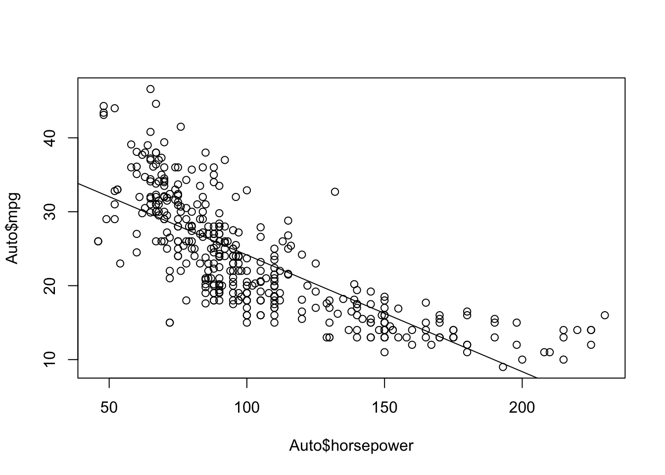

      

   3. par(mfrow = c(2, 2))
      plot(fit)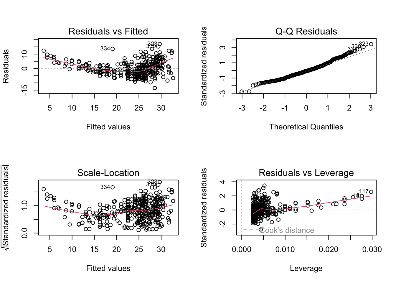

      

      There appears to be some trend in the residuals, indicating a linear fit is not appropriate.

2. Question

   set.seed(1)
   x <- rnorm(100)
   y <- 2 * x + rnorm(100)

   1. summary(lm(y ~ x + 0))

      
      Call:
      lm(formula = y ~ x + 0)
      
      Residuals:
          Min      1Q  Median      3Q     Max 
      -1.9154 -0.6472 -0.1771  0.5056  2.3109 
      
      Coefficients:
        Estimate Std. Error t value Pr(>|t|)    
      x   1.9939     0.1065   18.73   <2e-16 ***
      ---
      Signif. codes:  0 '***' 0.001 '**' 0.01 '*' 0.05 '.' 0.1 ' ' 1
      
      Residual standard error: 0.9586 on 99 degrees of freedom
      Multiple R-squared:  0.7798,    Adjusted R-squared:  0.7776 
      F-statistic: 350.7 on 1 and 99 DF,  p-value: < 2.2e-16

      Result is fairly close to what’s expected (2).

   2. summary(lm(x ~ y + 0))

      
      Call:
      lm(formula = x ~ y + 0)
      
      Residuals:
          Min      1Q  Median      3Q     Max 
      -0.8699 -0.2368  0.1030  0.2858  0.8938 
      
      Coefficients:
        Estimate Std. Error t value Pr(>|t|)    
      y  0.39111    0.02089   18.73   <2e-16 ***
      ---
      Signif. codes:  0 '***' 0.001 '**' 0.01 '*' 0.05 '.' 0.1 ' ' 1
      
      Residual standard error: 0.4246 on 99 degrees of freedom
      Multiple R-squared:  0.7798,    Adjusted R-squared:  0.7776 
      F-statistic: 350.7 on 1 and 99 DF,  p-value: < 2.2e-16

      Result is a bit far from what is expected (0.5), and it doesn’t land in its 95% confidence interval.

   3. The estimate in (a) is about 5 times the estimate in (b). The $t$-statistics, however, are identical.

   4. See: $$\begin{aligned} t &= \frac{\sum_{i} x_i y_i}{\sum_{j} x_j^2} \times \sqrt{\frac{(n-1)\sum_{j} x_j^2}{\sum_i (y_i - x_i \widehat{\beta})^2}} \\ &= \frac{\sqrt{n-1} \sum_i x_i y_i}{\sum_j x_j^2} \times \sqrt{\frac{\sum_j x_j^2}{\sum_i (y_i - x_i \widehat{\beta})^2}} \\ &= \frac{\sqrt{n-1} \sum_i x_i y_i}{\sqrt{\sum_j x_j^2}} \times \sqrt{\frac{1}{\sum_i (y_i - x_i \widehat{\beta})^2}} \\ &= \frac{\sqrt{n-1} \sum_i x_i y_i}{\sqrt{\sum_j x_j^2}} \times \sqrt{\frac{1}{\sum_i y_i^2 - 2y_i x_i \widehat{\beta} + x_i^2 \widehat{\beta}^2}} \\ &= \frac{\sqrt{n-1} \sum_i x_i y_i}{\sqrt{\sum_j x_j^2}} \times \sqrt{\frac{1}{\sum_i y_i^2 -2y_i x_i \frac{\sum_j x_j y_j}{\sum_k x_k^2} + x_i^2 (\frac{\sum_j x_j y_j}{\sum_k x_k^2})^2}} \\ &= \frac{\sqrt{n-1} \sum_i x_i y_i}{\sqrt{(\sum_i y_i^2)(\sum_j x_j^2) -2(\sum_i x_i y_i)^2 + (\sum_i x_i y_i)^2}} \\ &= \frac{\sqrt{n-1} \sum_i x_i y_i}{\sqrt{(\sum_i y_i^2)(\sum_j x^2_j) - (\sum_i x_i y_i)^2}} \end{aligned}$$

      In R, this is written as

      (sqrt(100 - 1) * sum(x * y)) / sqrt(sum(x^2) * sum(y^2) - sum(x * y)^2)

      [1] 18.72593

      This returns the same value as the t-statistic.

   5. Due to the symmetry of $x$ and $y$, we find we have the same formula as above. Hence the t-statistic is the same.

   6. fit <- lm(y ~ x)
      fit2 <- lm(x ~ y)
      summary(fit)

      
      Call:
      lm(formula = y ~ x)
      
      Residuals:
          Min      1Q  Median      3Q     Max 
      -1.8768 -0.6138 -0.1395  0.5394  2.3462 
      
      Coefficients:
                  Estimate Std. Error t value Pr(>|t|)    
      (Intercept) -0.03769    0.09699  -0.389    0.698    
      x            1.99894    0.10773  18.556   <2e-16 ***
      ---
      Signif. codes:  0 '***' 0.001 '**' 0.01 '*' 0.05 '.' 0.1 ' ' 1
      
      Residual standard error: 0.9628 on 98 degrees of freedom
      Multiple R-squared:  0.7784,    Adjusted R-squared:  0.7762 
      F-statistic: 344.3 on 1 and 98 DF,  p-value: < 2.2e-16

      summary(fit2)

      
      Call:
      lm(formula = x ~ y)
      
      Residuals:
           Min       1Q   Median       3Q      Max 
      -0.90848 -0.28101  0.06274  0.24570  0.85736 
      
      Coefficients:
                  Estimate Std. Error t value Pr(>|t|)    
      (Intercept)  0.03880    0.04266    0.91    0.365    
      y            0.38942    0.02099   18.56   <2e-16 ***
      ---
      Signif. codes:  0 '***' 0.001 '**' 0.01 '*' 0.05 '.' 0.1 ' ' 1
      
      Residual standard error: 0.4249 on 98 degrees of freedom
      Multiple R-squared:  0.7784,    Adjusted R-squared:  0.7762 
      F-statistic: 344.3 on 1 and 98 DF,  p-value: < 2.2e-16