Logistic Regression and Poisson Regression
Disclaimer
Some of the figures in this presentation are taken from “An Introduction to Statistical Learning, with applications in R” (Springer, 2021) with permission from the authors: G. James, D. Witten, T. Hastie and R. Tibshirani
Overview
- An overview of classification
- Logistic regression
- How to evaluate classification models
- Poisson regression
- Introduction to generalised linear models
Reading
James et al. (2021): Chapters 4.1, 4.2, 4.3, 4.6, 4.7.1, 4.7.2, 4.7.6, 4.7.7
An overview of classification
Regression vs. classification
Regression
- Y is quantitative
- Examples: Sales prediction, claim size prediction, stock price modelling
Classification
- Y is qualitative (or “categorial”, or “discrete”)
- Examples: fraud detection, face recognition, death
Some examples of classification problems
Success/failure of a treatment, explained by dosage of medicine administered, patient’s age, sex, BMI, severity of condition, etc.
Vote for/against political party, explained by age, gender, education level, region, ethnicity, geographical location, etc.
Customer churns/stays depending on usage pattern, complaints, social demographics, discounts offered, etc.
Example: Predicting defaults (Default from ISLR2)


default(Y) is a binary variable (yes/no as 1/0)- Annual
income(X_1) and credit cardbalance(X_2) are continuous predictors student(X_3) is a categorical predictor
Discussion: why not Linear Regression ?
- If we code the qualitative response as Y\in\{0,1\}, it becomes “numerical”.
- So, why not simply use (multiple) linear regression to predict Y from predictor(s) X_1,X_2,\ldots?
Simple linear regression on Default data:
Show code for Figure
mydefault <- ISLR2::Default
mydefault[, "numDefault"] <- 1
mydefault$numDefault[mydefault$default == "No"] <- 0
boxplot(lm(mydefault$numDefault ~ mydefault$balance + mydefault$student)$fitted.values,
        main="Fitted values of Default (1=Yes, 0=No)", col="lightgreen")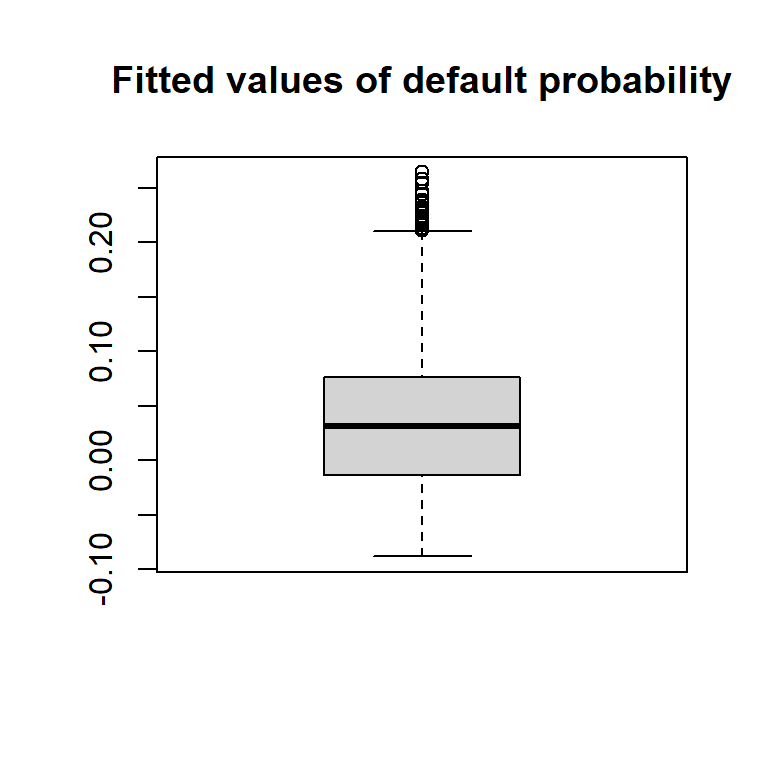
Classification problems
Coding in the binary case is simple Y \in \{0,1\} \Leftrightarrow Y\in\{{\color{#2171B5}\bullet},{\scriptsize{\color{#238B45}\blacksquare}}\}
Our objective is to find a good predictive model f that can:
- Estimate the probability \mathbb{P}(Y=1|X) \in [0, 1] as a certain f(X) f(X)\rightarrow [0,1] \Leftrightarrow {\color{#2171B5}\bullet}{\color{#6BAED6}\bullet}{\color{#BDD7E7}\bullet}{\color {#EFF3FF}\bullet}{\color{#EDF8E9}\bullet}{\color{#BAE4B3}\bullet}{\color{#74C476}\bullet}{\color {#238B45}\bullet}
- Classify observation f(X)\rightarrow \hat{Y}\in\{{\color{#2171B5}\bullet},{\scriptsize{\color{#238B45}\blacksquare}}\}
Logistic regression
Logistic Regression
- We are in the context of a binary response, Y \in \{0,1\}.
- We want to apply the ideas of linear regression to model Y, using predictors.
- Question for a Champion: why not simply model the probability \mathbb{P}[Y=1|\mathrm{X}] as function of predictor(s) \mathrm{X}?
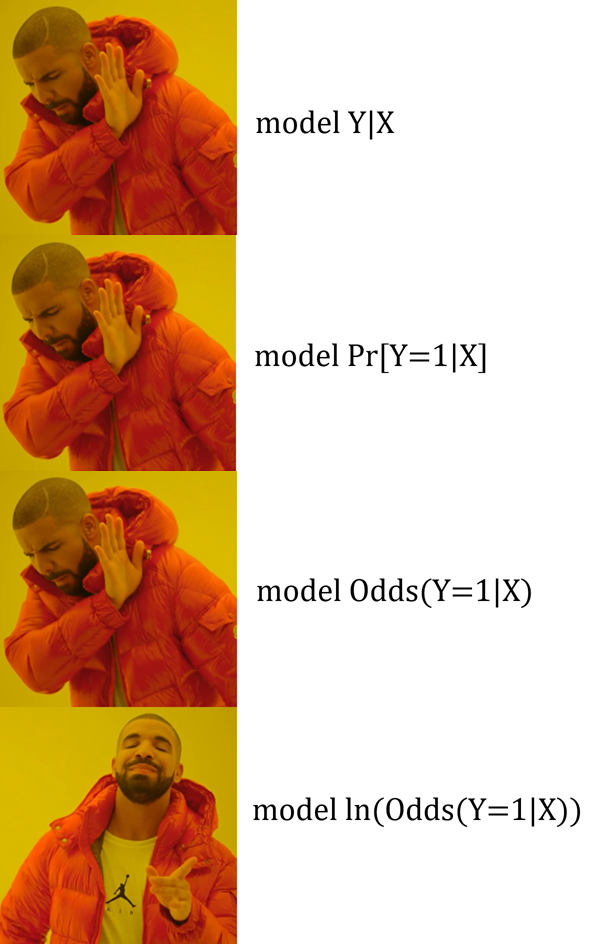
Principles of Logistic Regression I
The Odds of an event A measure the probability of A relative to its complement, i.e. \text{Odds}(A)=\frac{\mathbb{P}(A)}{\mathbb{P}(A^{\text{c}})} = \frac{\mathbb{P}(A)}{1-\mathbb{P}(A)}.
There is a “bijection” between probability and odds: if you know the probability you can find the odds, but also, if you know the odds you can recover the probability: \frac{1}{\text{Odds}(A)} = \frac{1}{\mathbb{P}(A)}-1. \mathbb{P}(A)=\frac{\text{Odds}(A)}{1+\text{Odds}(A)}.
Odds take values between 0 and \infty.
Principles of Logistic Regression II
- The main idea of logistic regression is to model the “log-odds” of Y=1 as a linear function of the predictor(s) \mathrm{X}.
- This is sensible because log-odds take values between -\infty and +\infty.
- The model is then:
\underbrace{\ln\left(\frac{\mathbb{P}(Y=1|\mathrm{X})}{1-\mathbb{P}(Y=1|\mathrm{X})}\right)}_{\text{log-odds}} = \underbrace{\beta_0 + \beta_1 X_1 + \cdots + \beta_p X_p}_{\text{linear model}}
In summary…
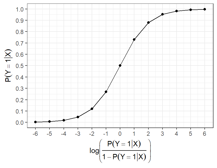
Probabilities, odds and log-odds
- We also have a bijection between probability and log-odds.
| probability | odds | logodds |
|---|---|---|
| 0.001 | 0.001 | -6.907 |
| 0.250 | 0.333 | -1.099 |
| 0.333 | 0.500 | -0.693 |
| 0.500 | 1.000 | 0.000 |
| 0.667 | 2.000 | 0.693 |
| 0.750 | 3.000 | 1.099 |
| 0.999 | 999.000 | 6.907 |
Logistic regression: interpretation of coefficients
- Recall that in multiple linear regression we modelled the response as
Y \approx \beta_0 + \beta_1 X_1 + \cdots + \beta_p X_p, \implies if predictor X_{j} increases by 1 we would predict Y to increase by {\beta}_j, on average.
- But now, our model is \begin{align*} \ln\left(\frac{\mathbb{P}(Y=1|\mathrm{X})}{1-\mathbb{P}(Y=1|\mathrm{X})}\right) & = \beta_0 + \beta_1 X_1 + \cdots + \beta_p X_p \\ \iff \text{Odds}(Y=1|\mathrm{X}) & = \mathrm{e}^{ \beta_0 + \beta_1 X_1 + \cdots + \beta_p X_p} \end{align*}
- I.e., in logistic regression, when X_j increases by 1, the log-odds of Y=1 increase by \beta_j.
- Equivalently, the odds (not the probabilities!) of Y=1 are multiplied by \mathrm{e}^{\beta_j}.
- Usually, we ultimately still care about the probability \mathbb{P}(Y=1|\mathrm{X}), given by
{\mathbb{P}}(Y=1|\mathrm{X}) = \frac{\mathrm{e}^{{\beta}_0 + {\beta}_1 X_1 + \cdots + {\beta}_p X_p}}{1+\mathrm{e}^{{\beta}_0 + {\beta}_1 X_1 + \cdots + {\beta}_p X_p}}.
- And we note that the “new probability” of Y=1 when X_j increases of 1 is \begin{align*} {\mathbb{P}}(Y=1|X_j \to X_j+1) = \frac{\mathrm{e}^{{\beta}_0 + {\beta}_1 X_1 + \cdots + {\beta}_j (X_j+1) +\cdots + {\beta}_p X_p}}{1+\mathrm{e}^{{\beta}_0 + {\beta}_1 X_1 + \cdots + {\beta}_j (X_j+1) +\cdots + {\beta}_p X_p}} & = \frac{\mathrm{e}^{\mathrm{X}{\boldsymbol{\beta}} } \cdot \mathrm{e}^{{\beta}_j}}{1+\mathrm{e}^{\mathrm{X}{\boldsymbol{\beta}}} \cdot \mathrm{e}^{{\beta}_j}}\\ & = \frac{\mathrm{e}^{\mathrm{X}{\boldsymbol{\beta}}}}{1+\mathrm{e}^{\mathrm{X}{\boldsymbol{\beta}}}+e^{-\beta_j}-1}. \end{align*}
- So, if \beta_j is positive, that probability increases (but not of a fixed amount \forall\,\mathrm{X}).
How are the coefficients estimated?
- In all the previous formulas, we assumed “known” coefficients \beta_j. In practice, we use (training) data and maximum-likelihood estimation to produce estimates \hat{\beta}_0, \hat{\beta}_1, \ldots \hat{\beta}_p.
- But note we never observe “probabilities”. Rather, we observe data y_1, y_2,\ldots y_n \in\{0,1\}, and associated predictors.
- We can still maximise the likelihood of this data, under our logistic regression model, and hence obtain the precious \hat{\beta}_js.
- Indeed, our model tells us that \mathbb{P}[Y_i=1|\boldsymbol{\beta},\mathrm{x}_i]=p(\mathrm{x}_i) = \frac{\mathrm{e}^{\mathrm{x}_i\boldsymbol{\beta}}}{1 + \mathrm{e}^{\mathrm{x}_i\boldsymbol{\beta}}} = \frac{1}{1 + \mathrm{e}^{-\mathrm{x}_i\boldsymbol{\beta}}}, where \mathrm{x}_i denotes the i’th row of the design matrix \boldsymbol{X}.
Log-likelihood
- Recalling that for Y\sim\text{Bernoulli}(p), the probability mass function is p^y (1-p)^{1-y}, \quad \text{for }y\in\{0,1\}, the likelihood of our data is L(\boldsymbol{\beta})= \prod_{i=1}^n \mathbb{P}[Y_i=y_i|\boldsymbol{\beta},\mathrm{x}_i] = \prod_{i=1}^n p(\mathrm{x}_i)^{y_i} (1-p(\mathrm{x}_i))^{1-{y_i}}.
- We can then maximise the log-likelihood: \ell (\boldsymbol{\beta}) = \sum_{i=1}^n y_i \ln p(\mathrm{x}_i) + (1-y_i) \ln(1- p(\mathrm{x}_i)).
- We take partial derivatives w.r.t. to each \beta_j and set to 0. This requires numerical methods (not covered here).
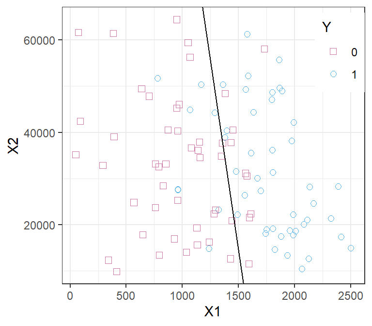
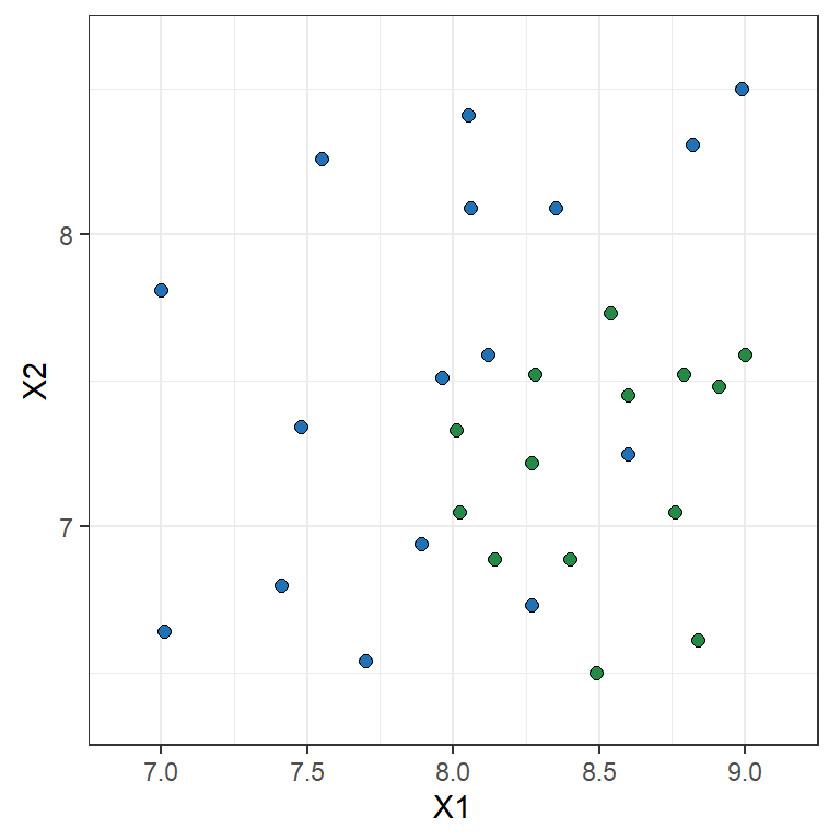
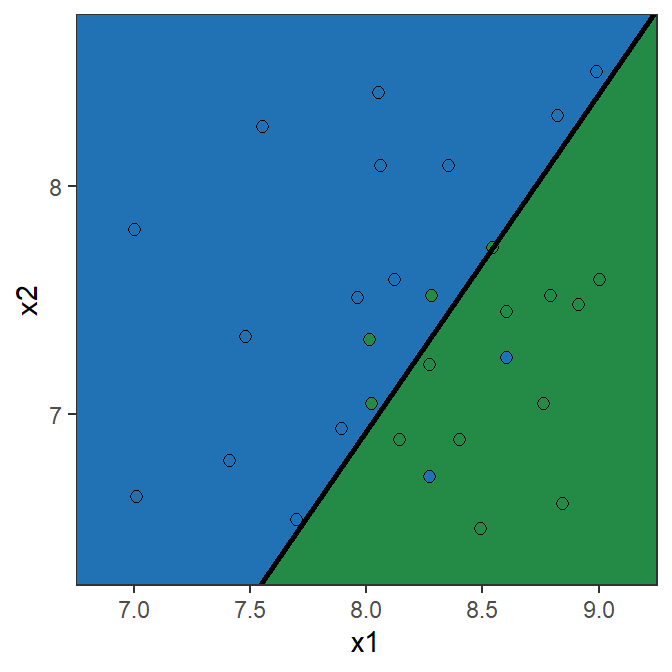
Toy example: Logistic Regression
Y = \begin{cases} 1 & \text{if } {\color{#2171B5}\bullet} \\ 0 & \text{if } {\scriptsize{\color{#238B45}\blacksquare}} \end{cases} \qquad \ln\left(\frac{\mathbb{P}(Y=1|X)}{1-\mathbb{P}(Y=1|X)}\right) = \beta_0 + \beta_1 X_1 + \beta_2 X_2
The parameter estimates are \hat{\beta}_0= 13.671, \hat{\beta}_1= -4.136, \hat{\beta}_2= 2.803
\hat{\beta}_1= -4.136 implies that the bigger X_1 the lower the chance it is a blue point
\hat{\beta}_2= 2.803 implies that the bigger X_2 the higher the chance it is a blue point

Toy example: Logistic Regression
\ln\left(\frac{\mathbb{P}(Y=1|X)}{1-\mathbb{P}(Y=1|X)}\right) = 13.671 - 4.136 X_1 + 2.803 X_2
| X1 | X2 | log-odds | P(Y=1|X) | prediction |
|---|---|---|---|---|
| 7.0 | 8.0 | 7.14 | 0.9992 | blue |
| 8.0 | 7.5 | 1.61 | 0.8328 | blue |
| 8.0 | 7.0 | 0.20 | 0.5508 | blue |
| 8.5 | 7.5 | -0.46 | 0.3864 | green |
| 9.0 | 7.0 | -3.93 | 0.0192 | green |
Note: the prediction is 1 (“blue”) if \mathbb{P}[Y=1|\mathrm{X}]>0.5.
Example: Predicting defaults
glmStudent <- glm(default ~ student, family = binomial(), data = ISLR2::Default)
summary(glmStudent)
Call:
glm(formula = default ~ student, family = binomial(), data = ISLR2::Default)

Coefficients:
            Estimate Std. Error z value Pr(>|z|)
(Intercept) -3.50413    0.07071  -49.55  < 2e-16 ***
studentYes   0.40489    0.11502    3.52 0.000431 ***
---
Signif. codes:  0 '***' 0.001 '**' 0.01 '*' 0.05 '.' 0.1 ' ' 1

(Dispersion parameter for binomial family taken to be 1)

    Null deviance: 2920.6  on 9999  degrees of freedom
Residual deviance: 2908.7  on 9998  degrees of freedom
AIC: 2912.7

Number of Fisher Scoring iterations: 6
Example: Predicting defaults
glmAll <- glm(default ~ balance + income + student, family = binomial(), data = ISLR2::Default)
summary(glmAll)
Call:
glm(formula = default ~ balance + income + student, family = binomial(),
    data = ISLR2::Default)

Coefficients:
              Estimate Std. Error z value Pr(>|z|)
(Intercept) -1.087e+01  4.923e-01 -22.080  < 2e-16 ***
balance      5.737e-03  2.319e-04  24.738  < 2e-16 ***
income       3.033e-06  8.203e-06   0.370  0.71152
studentYes  -6.468e-01  2.363e-01  -2.738  0.00619 **
---
Signif. codes:  0 '***' 0.001 '**' 0.01 '*' 0.05 '.' 0.1 ' ' 1

(Dispersion parameter for binomial family taken to be 1)

    Null deviance: 2920.6  on 9999  degrees of freedom
Residual deviance: 1571.5  on 9996  degrees of freedom
AIC: 1579.5

Number of Fisher Scoring iterations: 8
Example: Predicting defaults - Discussion
Results of logistic regression:
default against student
| Predictor | Coefficient | Std error | Z-statistic | P-value |
|---|---|---|---|---|
(Intercept) |
-3.5041 | 0.0707 | -49.55 | <0.0001 |
student = Yes |
0.4049 | 0.1150 | 3.52 | 0.0004 |
default against balance, income, and student
| Predictor | Coefficient | Std error | Z-statistic | P-value |
|---|---|---|---|---|
(Intercept) |
-10.8690 | 0.4923 | -22.080 | < 0.0001 |
balance |
0.0057 | 2.319e-04 | 24.738 | < 0.0001 |
income |
3.033e-06 | 8.203e-06 | 0.370 | 0.71152 |
student = Yes |
-0.6468 | 0.2362 | -2.738 | 0.00619 |
How to evaluate classification models
Error rate and accuracy in classification problems
- Recall the (training) error rate is simply \text{error rate}=\frac{1}{n}\sum_{i=1}^n I(y_i\neq \hat{y}_i)
- In our toy example (with a 50% threshold), \text{training error rate}= \frac{6}{30} = 0.2
- We call accuracy “1-\text{error rate}”; this represents the proportion of correct predictions.
- Question for a Champion: is the error rate enough to evaluate the performance of a model?

There are two types or errors we can make!

Confusion matrix and Recall
- The confusion matrix of the fitted model gives us a more complete picture.
| Y=0 | Y=1 | Total | |
|---|---|---|---|
| \hat{Y}=0 | TN | FN | Predicted N |
| \hat{Y}=1 | FP | TP | Predicted P |
| Total | Actually N | Actually P | n |
- \text{TP Rate} = \text{Recall} = \frac{\text{TP}}{\text{Actually P}}
- In words: of all items actually positive, what proportion is predicted to be positive.
- Analogy: out of all actual criminals that are trialed, what proportion are declared guilty.
- \text{FN Rate} = 1-\text{Recall} = \frac{\text{FN}}{\text{Actually P}}
Specificity
\text{TN Rate} = \text{Specificity} = \frac{\text{TN}}{\text{Actually N}}
In words: of all items actually negative, what proportion is predicted to be negative.
Analogy: out of all innocent people that are trialed, what proportion are declared “not guilty”.
\text{FP Rate} = 1-\text{Specificity} = \frac{\text{FP}}{\text{Actually N}}
Precision
- When evaluating classification models, Precision is another common metric used. It is defined as \text{Precision} = \frac{\text{TP}}{\text{Predicted P}}
- In words: of all items predicted to be positive, what proportion are actually positive.
- Analogy: out of all people trialed and “declared guilty”, what proportion is actually guilty.
- Prioritising precision means we care about the reliability of positive predictions, which typically involves reducing false positives.
- Question for a Champion: why is precision useful, given we already have the notion of specificity (1- \text{FP Rate})?
Precision: example
- Careful that precision can be low even if specificity is high! This is something to watch out for especially in the case of unbalanced data (i.e., when one category is much more likely than the other).
- Fictional example: a lecturer is investigating cheating in an exam. Y=1 means a student actually cheated (Y=0 means they did not) and \hat{Y}=1 means the lecturer convicts a student of cheating. The findings are summarised below… are those results “good”?
| Y=0 | Y=1 | Total | |
|---|---|---|---|
| \hat{Y}=0 | 969 | 1 | 970 |
| \hat{Y}=1 | 21 | 9 | 30 |
| Total | 990 | 10 | 1000 |
- Accuracy: 97.8%; Recall: 90%; Specificity: 97.9%
- Precision:
Confusion matrix: Toy example (50% Threshold)
Confusion matrix
Y=0 Y=1 Total \hat{Y}=0 10 2 12 \hat{Y}=1 4 14 18 Total 14 16 30 \text{Recall} = \frac{14}{16}=0.875
\text{Specificity} = \frac{10}{14}=0.714
\text{Precision} = \frac{14}{18}=0.778

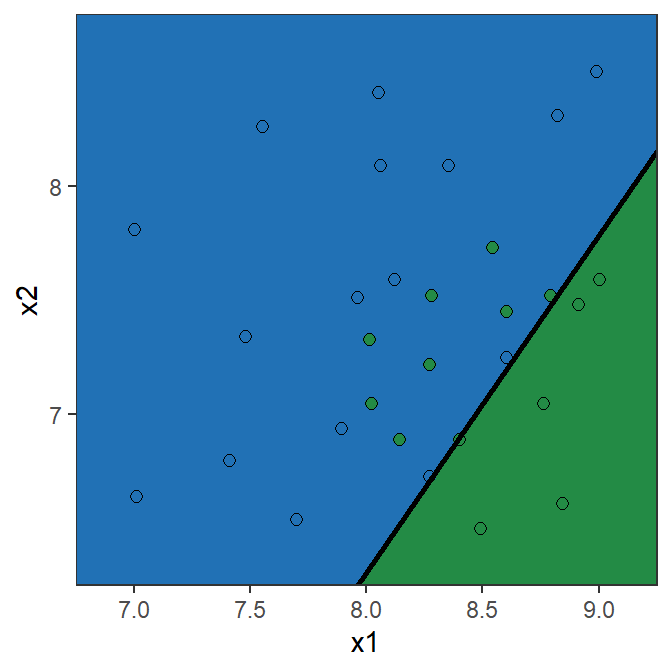
Confusion matrix: Toy example (15% Threshold)
Confusion matrix
Y=0 Y=1 Total \hat{Y}=0 6 0 6 \hat{Y}=1 8 16 24 Total 14 16 30 \text{Recall} = \frac{16}{16}=1
\text{Specificity} = \frac{6}{14}=0.429
\text{Precision} = \frac{16}{24}=0.667
ROC Curve and AUC: Toy example
- ROC Curve: plots the true-positive rate against the false-positive rate.
- A good model will have its ROC curve hugging the top-left corner.
- AUC is the area under the ROC curve: for this toy example \text{AUC=} 0.8929.
Poisson regression
Poisson regression - Motivation
In many applications we need to model count data, Y\in\{0,1,2,3,\ldots\}:
In mortality studies and/or health insurance, the aim is to explain the number of deaths and/or disabilities in terms of predictor variables such as age, gender, occupation and lifestyle.
In general insurance, the count of interest may be the number of claims made on vehicle insurance policies. This could be a function of the driver’s characteristics, the geographical location of driver, the age of the car, type of car, previous claims experience, and so on.
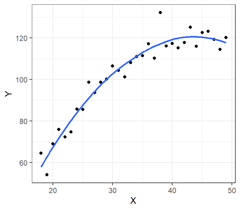
The Bikeshare dataset - Discussion

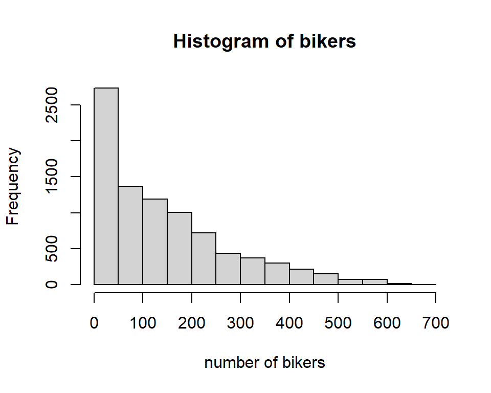

Why not use muliple linear regression?
Y = \beta_0 + \beta_1 X_1 + \cdots + \beta_p X_p + \epsilon
- Could predict negative values.
- Constant variance assumption of errors may be inadequate.
- Assumes continuous numbers while counts are integers.
\log(Y) = \beta_0 + \beta_1 X_1 + \cdots + \beta_p X_p + \epsilon
- Solves problem of negative values.
- Not applicable with zero counts.
- Can help with the “constant variance” problem.
- Still assumes a continuous response, while the log of a count is not continuous.
Poisson regression
- Assume that Y \sim \text{Poisson}(\lambda),
\mathbb{P}(Y=k) = \frac{e^{-\lambda}\lambda^k}{k!} \quad \text{for } k=0,1,2,\ldots \quad \text{with } \mathbb{E}[Y]= \text{Var}(Y)=\lambda.
- We let \lambda depend on the predictors in the following way:
\log(\lambda(X_1,\ldots,X_p)) = \beta_0 + \beta_1 X_1 + \cdots + \beta_p X_p.
Hence, \mathbb{E}[Y] = \lambda(X_1,X_2,\ldots, X_p) = \mathrm{e}^{\beta_0 + \beta_1 X_1 + \cdots + \beta_p X_p}.
This is convenient because \lambda cannot be negative.
Interpretation: an increase in X_j by one unit is associated with a change in \mathbb{E}[Y] by a multiplicative factor e^{\beta_j}.
Comments about Poisson regression
- Using the data and maximum likelihood estimation, obtain \hat{\beta}_0, \hat{\beta}_1, \ldots \hat{\beta}_p
L(\beta_0,\beta_1,\ldots,\beta_p)=\prod_{i=1}^n\frac{e^{-\lambda(\mathrm{x}_i)}\lambda(\mathrm{x}_i)^{y_i}}{y_i!} \quad \text{with} \quad \lambda(\mathrm{x}_i) = \mathrm{e}^{\beta_0 + \beta_1 x_{i1} + \cdots + \beta_p x_{ip}}
- Mean-variance relationship: \mathbb{E}[Y]= \text{Var}(Y)=\lambda \, implies that the variance is non-constant and increases with the mean.
- Fitted values \hat{y}_i are simply set as the estimated means \hat{\lambda}_i, hence are always positive.
- We don’t have an exact equivalent of the R^2 from linear regression (because we don’t have the nice identity \text{TSS}=\text{MSS}+\text{RSS}).
- We can use the AIC to compare models. Then, deciding to add / remove predictors can be done as in linear regression.
- Most of the modelling limitations of linear regression (e.g., collinearity) carry over as well.
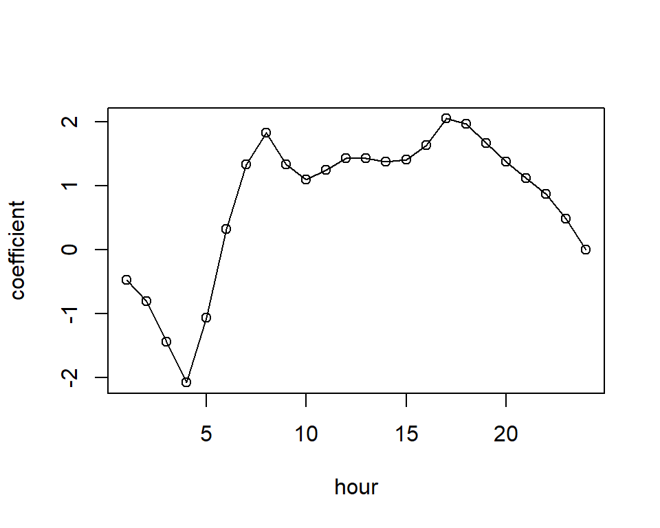
Poisson regression - Bikeshare dataset
plot(x = 1:12, y = c(0, glmBikeshare$coefficients[7:17]), type = 'o',
     xlab = "month", ylab = "coefficient", xaxt = "n")
axis(1, at=1:12, labels=substr(month.name, 1, 1))
plot(x = 1:24, y = c(glmBikeshare$coefficients[18:40], 0), type = 'o',
     xlab = "hour", ylab = "coefficient")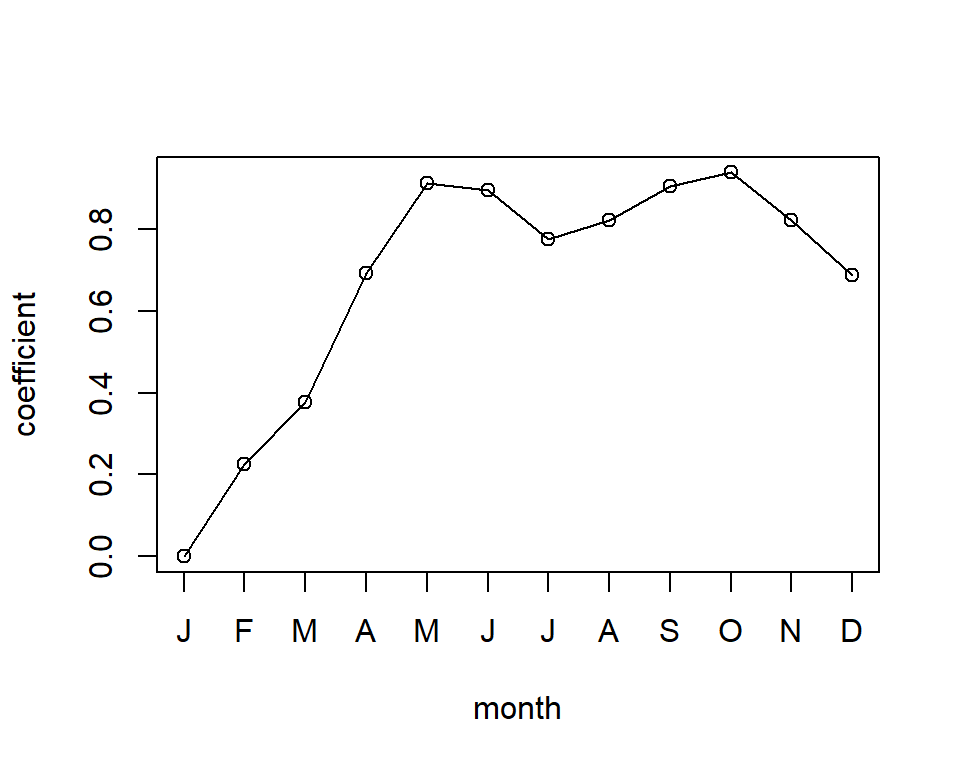
Generalised linear models
Generalised linear models
| Linear Regression | Logistic Regression | Poisson Regression | Generalised Linear Models | |
|---|---|---|---|---|
| Type of Data | Continuous | Binary (Categorical) | Count | Flexible |
| Use | Prediction of continuous variables | Classification | Prediction of an integer number | Flexible |
| Distribution of Y|\mathrm{x} | Normal | Bernoulli (Binomial for multiple trials) | Poisson | Exponential Family |
| \mathbb{E}[Y|\mathrm{X}] | \mathrm{X}\boldsymbol{\beta} | \frac{e^{\mathrm{X}\boldsymbol{\beta}}}{1+e^{\mathrm{X}\boldsymbol{\beta}}} | e^{\mathrm{X}\boldsymbol{\beta}} | g^{-1}(\mathrm{X}\boldsymbol{\beta}) |
| Link Function Name | Identity | Logit | Log | Depends on the choice of distribution |
| Link Function Expression | g(\mu) = \mu | g(\mu) = \log \left(\frac{\mu}{1-\mu}\right) | g(\mu) = \log(\mu) | Depends on the choice of distribution |
References
James, G., Witten, D., Hastie, T., & Tibshirani, R. (2021). An Introduction to Statistical Learning: with Applications in R. Springer.
Comments about logistic regression