Lab 4: Logistic Regression

Questions

Conceptual Questions

\star Solution (ISLR2, Q4.6) Suppose we collect data for a group of students in a statistics class with variables X_1=hours studied, X_2= undergrad GPA, and Y= receive an A. We fit a logistic regression and produce estimated coefficient, \hat{\beta}_0 = -6, \hat{\beta}_1 = 0.05, \hat{\beta}_2 = 1.
1. Estimate the probability that a student who studies for 40 h and has an undergrad GPA of 3.5 gets an A in the class.
2. How many hours would the student in part (a) need to study to have a 50% chance of getting an A in the class?
Solution (ISLR2, Q4.7) Suppose that we wish to predict whether a given stock will issue a dividend this year (“Yes” or “No”) based on X, last year’s percent profit. We examine a large number of companies and discover that the mean value of X for companies that issued a dividend was \bar{X} = 10 (which means 10\%) while the mean for those that didn’t was \bar{X} = 0. In addition, the variance of X for both these sets of companies was \hat{\sigma}^2 = 36. Finally, 80\% of companies issued dividends. Assuming that X follows a Normal distribution, predict the probability that a company will issue a dividend this year given that its percentage profit was X = 4 last year.

Hint: Recall that the density function for a normal random variable is f(x) = \frac{1}{\sqrt{2\pi\sigma^2}} \mathrm{e}^{-(x-\mu)^2/2\sigma^2}. You will need to use Bayes’ theorem.
\star Solution (ISLR2, Q4.8) Suppose that we take a data set, divide it into equally-sized training and test sets, and then try out two different classification procedures. First we use logistic regression and get an error rate of 20% on the training data and 30% on the test data. Next we use 1-nearest neighbors (i.e. K = 1) and get an average error rate (averaged over both test and training data sets) of 18%. Based on these results, which method should we prefer to use for classification of new observations? Why?
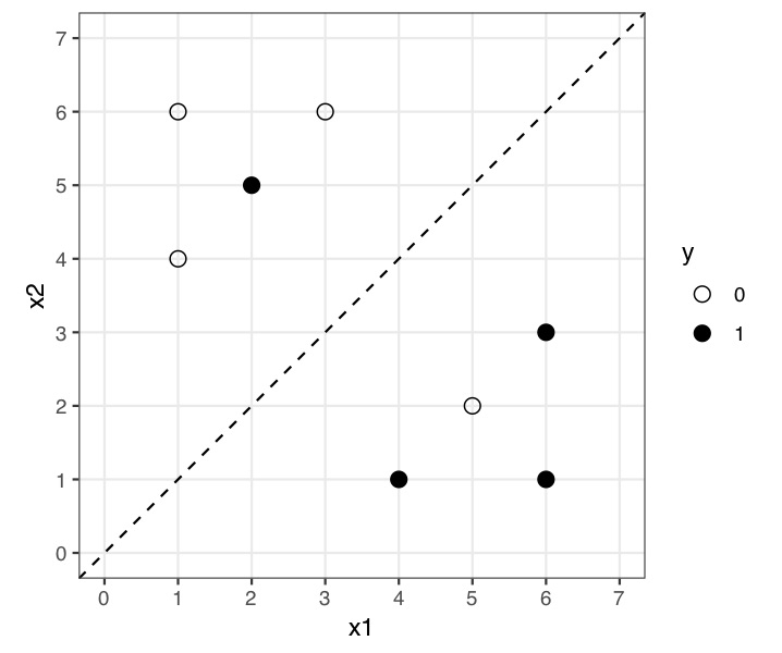
\star Solution Consider a classification problem with two continuous inputs, x_1 and x_2, and a binary (0/1) target variable, y. There are 8 training cases, plotted in the following figure.

Cases where y=1 (positive cases) are plotted as black dots and cases where y=0 (negative cases) as white dots, with the location of the dot giving the inputs, x_1 and x_2, for that training case. A logistic regression has been fitted to these data with estimated regression equation:

\begin{align*} \log \left(\frac{\mathbb{P}(Y=1|x_1, x_2)}{1-\mathbb{P}(Y=1|x_1, x_2)} \right) = x_1 - x_2 . \end{align*}

The corresponding classification decision boundary using a threshold of 0.5 probability is given by x_2=x_1 and is represented by the dashed line in the figure (an observation is assigned to class y=1 if \mathbb{P}(Y=1|x_1,x_2)>0.5).
1. Explain why any data point such that x_1>x_2 (i.e., on the right of the decision boundary), will be assigned the class y=1.
2. Fill in the confusion matrix below (find A, B, C and D) and compute the total error rate, the error rate given class 1 and the error rate given class 0.
  
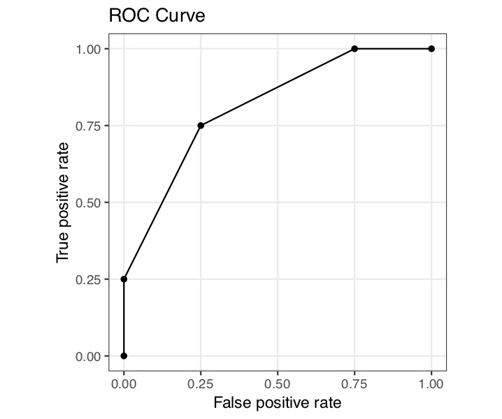
  True y=0 True y=1 Total
  
  Fitted y=0 A B 4
  
  Fitted y=1 C D 4
  
  Total 4 4 8
3. Draw a ROC curve for the logistic regression depicted in the above Figure.
Solution Consider a set-up for logistic regression with only one predictor (and a response Y\in\{0,1\}).
1. Using log-likelihood, derive two equations that, if solved for \beta_0 and \beta_1, would provide the MLEs of the logistic regression model. Hint: recall that in logistic regression we have \mathbb{P}[Y_i=1|\mathrm{x}_i]=\frac{\mathrm{e}^{\mathrm{x}_i\boldsymbol{\beta}}}{1+\mathrm{e}^{\mathrm{x}_i\boldsymbol{\beta}}}.
2. Using the results from the previous question, show that under MLE the expected number of “class y=1” matches the observed number of “class y=1”.

Applied Questions

\star Solution (ISLR2, Q4.13) This question should be answered using the Weekly data set, which is part of the ISLR2 package. This data is similar in nature to the Smarket data from this chapter’s lab, except that it contains 1,089 weekly returns for 21 years, from the beginning of 1990 to the end of 2010.
1. Produce some numerical and graphical summaries of the Weekly data. Do there appear to be any patterns?
2. Use the full data set to perform a logistic regression with Direction as the response and the five lag variables plus Volume as predictors. Use the summary function to print the results. Do any of the predictors appear to be statistically significant? If so, which ones?
3. Compute the confusion matrix and overall fraction of correct predictions. Explain what the confusion matrix is telling you about the types of mistakes made by logistic regression.
4. Now fit the logistic regression model using a training data period from 1990 to 2008, with Lag2 as the only predictor. Compute the confusion matrix and the overall fraction of correct predictions for the held out data (that is, the data from 2009 and 2010).
5. Repeat (d) using KNN with K = 1.
6. Which of these methods appears to provide the best results on this data?
7. Experiment with different combinations of predictors, including possible transformations and interactions, for each of the methods. Report the variables, method, and associated confusion matrix that appears to provide the best results on the held out data. Note that you should also experiment with values for K in the KNN classifier.
\star Solution (ISLR2, Q4.14) In this problem, you will develop a model to predict whether a given car gets high or low gas mileage based on the Auto data set.
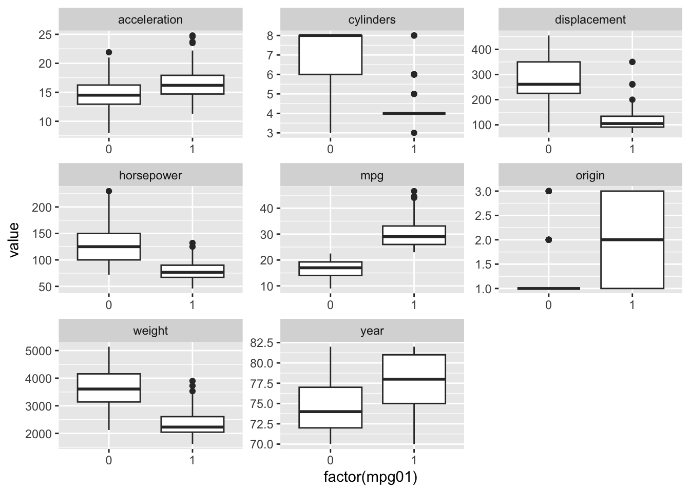
1. Create a binary variable, mpg01, that contains a 1 if mpg contains a value above its median, and a 0 if mpg contains a value below its median. You can compute the median using the median() function. Note you may find it helpful to use the data.frame() function to create a single data set containing both mpg01 and the other Auto variables.
2. Explore the data graphically in order to investigate the association between mpg01 and the other features. Which of the other features seem most likely to be useful in predicting mpg01? Scatterplots and boxplots may be useful tools to answer this question. Describe your findings.
3. Split the data into a training set and a test set.
4. Perform logistic regression on the training data in order to predict mpg01 using the variables that seemed most associated with mpg01 in (b). What is the test error of the model obtained?
5. Perform KNN on the training data, with several values of K, in order to predict mpg01. Use only the variables that seemed most associated with mpg01 in (b). What test errors do you obtain? Which value of K seems to perform the best on this data set?

Solutions

Conceptual Questions

Question
1. \frac{\exp(-6+0.05 \times 40 + 1 \times 3.5 )}{1+\exp(-6+0.05 \times 40 + 1 \times 3.5 )} = 0.378
2. \exp(-6 + 0.05x_1 + 3.5) = \frac{0.5}{1-0.5} \implies x_1 = 50
Question Denote “Yes” as class 1, and “No” as class 0. Then, we have \mu_1 = 10, \mu_0 = 0, \sigma^2=36. We see: \begin{aligned} \mathbb{P}(Y=1|X=4) &= \frac{\mathbb{P}(Y=1,X=4)}{\mathbb{P}(X=4)} \\ &= \frac{\mathbb{P}(X=4|Y=1)\mathbb{P}(Y=1)}{\mathbb{P}(X=4|Y=1)\mathbb{P}(Y=1)+\mathbb{P}(X=4|Y=0)\mathbb{P}(Y=0)} \\ &= \frac{0.8\frac{1}{\sqrt{2\pi\times 36}} \mathrm{e}^{-(4-10)^2/(2\times 36)}} {\frac{1}{\sqrt{2\pi\times 36}}\left( 0.8\mathrm{e}^{-(4-10)^2/(2\times 36)} + 0.2\mathrm{e}^{-(4-0)^2/(2\times 36)} \right)} \\ &= 0.7518525 \end{aligned}
Question One-nearest neighbours perfectly fits the training data, so the training error rate will be 0%. Hence, the test error rate is 36%, since the test and training sets are equally sized. Since the logistic model has a lower test error rate of 30%, we prefer this model.
Question
1. Recall that \text{odds}=\text{proba}/(1-\text{proba}). So, a point will be assigned the class y=1 if its odds of y=1 are >1 (which corresponds to its probability being >0.5). Equivalently, its log-odds must be >\ln(1), i.e., greater than 0. Hence, a point will be assigned the class y=1 if
\ln(\text{odds}) > 0 \iff x_1 - x_2 > 0 \iff x_1 > x_2.
1. For a decision boundary at 0.5, the majority within each regions will be predicted for that training data. Hence, anything “above the line” will be predicted as y=0, and anything below will be predicted as y=1. This leads to 3 true positives for y=0, 1 false positive for y=0. And similarly for y=1, 3 true positives for y=1, and 1 false positive for y=1. Hence, we have A = 3, B = 1, C = 1, D = 3. The total error rate is \frac{2}{8} = 0.25, and the error rate |_{y=1} = \frac{1}{4} = 0.25, and error rate |_{y=0} = \frac{1}{4} = 0.25.
2. To plot the ROC curve, we can change the threshold. You can imagine changing the threshold as moving the decision boundary up and down. As we move this up and down, we would get changing true positive and false positive rates. See the figure below.
Question
1. Let \mathbb{P}(Y_i=1 | x_i;\beta_0,\beta_1)=p(x_i,\beta_0,\beta_1). The log likelihood is \begin{aligned} l(\beta_0,\beta_1) &= \sum_{i=1}^N\left( y_i\log p(x_i,\beta_0,\beta_1)+(1-y_i)\log(1-p(x_i,\beta_0,\beta_1))\right) \\ &= \sum_{i=1}^N\left( y_i(\beta_0+\beta_1x_i)-\log(1+\mathrm{e}^{\beta_0+\beta_1x_i}))\right) . \end{aligned} The score function is then derived by differentiating and setting to zero: \frac{\partial l(\beta_0,\beta_1)}{\partial\beta_0}=\sum_{i=1}^N(y_i-p(x_i,\beta_0,\beta_1))=0 \,, \frac{\partial l(\beta_0,\beta_1)}{\partial\beta_1}=\sum_{i=1}^Nx_i(y_i-p(x_i,\beta_0,\beta_1))=0 \,.
2. The expected number of 1’s is just the sum of the expected values of individual Y_i’s. But recall that the expected value of a Bernoulli(p) is simply p. Hence, we have \sum_{i=1}^N \mathbb{E}(Y_i=1|x_i) = \sum_{i=1}^N p(x_i,\beta_0,\beta_1) = \sum_{i=1}^N y_i \,, where the last equality comes from the first of the score functions in the previous part, \sum_{i=1}^N(y_i-p(x_i,\beta_0,\beta_1))=0 \,.

Applied Questions

Question

The volume has increased over time. Everything else seems largely uncorrelated. More details are available p171-172 of the book.

library(ISLR2)
library(MASS)

fit <- glm(Direction ~ Lag1 + Lag2 + Lag3 + Lag4 + Lag5 + Volume,
  family = "binomial", data = Weekly
)
summary(fit)


Call:
glm(formula = Direction ~ Lag1 + Lag2 + Lag3 + Lag4 + Lag5 + 
    Volume, family = "binomial", data = Weekly)

Coefficients:
            Estimate Std. Error z value Pr(>|z|)   
(Intercept)  0.26686    0.08593   3.106   0.0019 **
Lag1        -0.04127    0.02641  -1.563   0.1181   
Lag2         0.05844    0.02686   2.175   0.0296 * 
Lag3        -0.01606    0.02666  -0.602   0.5469   
Lag4        -0.02779    0.02646  -1.050   0.2937   
Lag5        -0.01447    0.02638  -0.549   0.5833   
Volume      -0.02274    0.03690  -0.616   0.5377   
---
Signif. codes:  0 '***' 0.001 '**' 0.01 '*' 0.05 '.' 0.1 ' ' 1

(Dispersion parameter for binomial family taken to be 1)

    Null deviance: 1496.2  on 1088  degrees of freedom
Residual deviance: 1486.4  on 1082  degrees of freedom
AIC: 1500.4

Number of Fisher Scoring iterations: 4

It looks like Lag2 is significant.

fit$y[1] # check how R is encoding "Up" and "Down"

1 
0

pred <- rep("Up", length(Weekly$Direction))
pred[fit$fitted.values < 0.5] <- "Down"
table(pred, actual=Weekly$Direction)

      actual
pred   Down  Up
  Down   54  48
  Up    430 557

There is a problem in that it is allocating too many observations to Up in the above confusion matrix when they should be Down (430 on false-positive). The false-negative rate is low but that is because the negative rate in general is too low.

train <- (Weekly$Year <= 2008)
fit2 <- glm(Direction ~ Lag2, family = "binomial", data = Weekly, subset = train)
pred.fit2 <- predict(fit2, newdata = Weekly[!train, ], type = "response")
pred.val <- rep("Down", length(pred.fit2))
pred.val[pred.fit2 > 0.5] <- "Up"
table(pred.val, actual=Weekly$Direction[!train])

        actual
pred.val Down Up
    Down    9  5
    Up     34 56

library(class)
train.knn <- Weekly$Lag2[train]
test.knn <- as.matrix(Weekly[!train, "Lag2"], ncol = 1)
train.knn.result <- Weekly[train, "Direction"]

set.seed(1)
fit5 <- knn(train=train.knn, test=test.knn, cl=train.knn.result, k=1)
table(fit5, actual=Weekly$Direction[!train])

      actual
fit5   Down Up
  Down   21 30
  Up     22 31

Logistic regression has a (poor) test error rate of (5+34)/104 = 37.5\%, while KNN with K = 1 has a quite terrible error rate of at (30+22)/104=50\% (exactly what you would get by flipping a coin!). Overall, both models are quite bad, but in different ways. Logistic regression too easily predicts “Up”, and so has a very high “false positive” rate (34/43\approx 79\%), but also a low “false negative” rate (5/61\approx 8\%). KNN has a better (but still bad) “false positive” rate (22/43 \approx 51\%) and an equally bad “false negative” rate (30/61 \approx 49\%). Both models are bad, but if we have to pick we would probably go with logistic regression here.

Question

myAuto <- Auto
myAuto["mpg01"] <- rep(0, length(myAuto$mpg))
myAuto[myAuto$mpg > median(myAuto$mpg), "mpg01"] <- 1
summary(myAuto$mpg01)

   Min. 1st Qu.  Median    Mean 3rd Qu.    Max. 
    0.0     0.0     0.5     0.5     1.0     1.0

# pairs(myAuto) # doesn't work well since mpg01 is 0 or 1

Use commands such as boxplot(myAuto$<COLUMN NAME>~myAuto$mpg01) to produce the required plots. Alternatively, you can use the following commands.

suppressMessages(library(tidyverse))
plotData <- myAuto %>%
  keep(is.numeric) %>%
  gather(variable, value, -mpg01)
ggplot(plotData) +
  geom_boxplot(aes(x = factor(mpg01), y = value)) +
  facet_wrap(~variable, scales = "free")

Cylinders, displacement, horsepower and weight look like they could predict mpg01, as there distributions vary a lot depending on whether mpg01 =0 or =1.

```
1set.seed(1)
2train.set <- sample(length(myAuto$mpg), length(myAuto$mpg) / 2)
3train <- (seq(1, length(myAuto$mpg)) %in% train.set)
```
1

Use this seed to get the same results as the solutions

2

sample creates a random vector of integers, of specified size (length(myAuto$mpg)/2) from the elements of the vector 1 2 3 ... length(myAuto$mpg).

3

Create a vector of TRUE or FALSE, to indicate if a given observation is in the training set or not.

fit3 <- glm(mpg01 ~ cylinders + origin + displacement + weight,
  family = "binomial",
  data = myAuto, subset = train
)
pred.fit3 <- predict(fit3, newdata = myAuto[!train, ], type = "response")
pred.val3 <- rep(0, length(pred.fit3))
pred.val3[pred.fit3 > 0.5] <- 1
table(pred.val3, actual=myAuto$mpg01[!train]) # confusion matrix

         actual
pred.val3  0  1
        0 86  7
        1 16 87

100 * mean(pred.val3 != myAuto$mpg01[!train]) # test error rate

[1] 11.73469

100 * (16 + 7) / (86 + 7 + 16 + 87) # test error rate check

[1] 11.73469

The test error in this case is equal to 11.73\%.

set.seed(1)
train.knn <- myAuto[train, c("cylinders", "origin", "displacement", "weight")]
test.knn <- myAuto[!train, c("cylinders", "origin", "displacement", "weight")]
train.knn.result <- myAuto[train, "mpg01"]
error.rates <- c()
for (i in 1:10){
  fit5 <- knn(train.knn, test.knn, train.knn.result, k = i)
  mytable <- table(fit5, myAuto[!train, "mpg01"])
  error.rates[i] <- (mytable[2] + mytable[3]) / sum(mytable) * 100
}
cbind(K=1:10, error.rates) # error rates

       K error.rates
 [1,]  1    17.85714
 [2,]  2    15.81633
 [3,]  3    12.24490
 [4,]  4    13.26531
 [5,]  5    12.24490
 [6,]  6    12.75510
 [7,]  7    12.24490
 [8,]  8    11.73469
 [9,]  9    12.24490
[10,] 10    12.24490

min(error.rates) # min error rate, check corresponding k

[1] 11.73469

The best test error rate is obtained with K=8, at 11.73\% (exactly the same as in logistic regression). Hence, it’s hard to pick the “best” method in this case.

Question for a Champion: if we change the “seed” in the above code, the results will change a bit, but only for even values of K… why is that?

	True y=0	True y=1	Total
Fitted y=0	A	B	4
Fitted y=1	C	D	4
Total	4	4	8