library(ISLR2)
set.seed(1)
train.set <- sample(nrow(Carseats), nrow(Carseats) / 2)
train <- 1:nrow(Carseats) %in% train.setLab 8: Tree-based Methods
Questions
Conceptual Questions
\star Solution (ISLR2, Q8.3) Consider the Gini index, classification error, and entropy in a simple classification setting with two classes. Create a single plot that displays each of these quantities as a function of \hat{p}_{m1}. The x-axis should display \hat{p}_{m1}, ranging from 0 to 1, and the y-axis should display the value of the Gini index, classification error, and entropy.
Hint: In a setting with two classes, \hat{p}_{m1} = 1 - \hat{p}_{m2}. You could make this plot by hand, but it will be much easier to make in
R.\star Solution (ISLR2, Q8.4) This question relates to the plots in the textbook Figure 8.14, reproduced here as Figure 1:
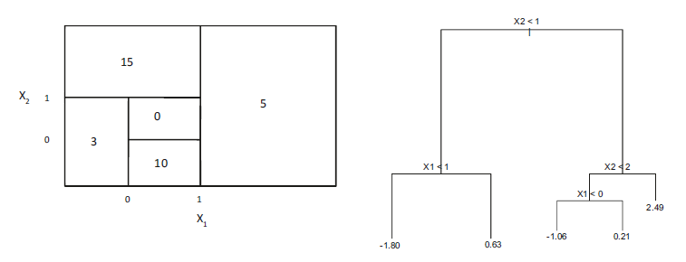
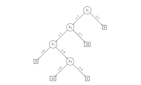
Figure 1: Left: A partition of the predictor space corresponding to Exercise 4a. Right: A tree corresponding to Exercise 4b. Sketch the tree corresponding to the partition of the predictor space illustrated in the left-hand panel of Figure 8.14. The numbers inside the boxes indicate the mean of Y within each region.
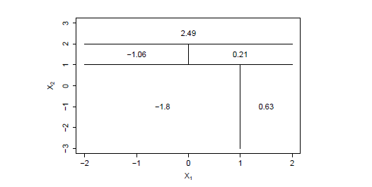
Create a diagram similar to the left-hand panel of Figure 8.14, using the tree illustrated in the right-hand panel of the same figure. You should divide up the predictor space into the correct regions, and indicate the mean for each region.
\star Solution (ISLR2, Q8.5) Suppose we produce ten bootstrapped samples from a data set containing red and green classes. We then apply a classification tree to each bootstrapped sample and, for a specific value of X, produce 10 estimates of \mathbb{P}(\text{Class is Red}|X): 0.1, 0.15, 0.2, 0.2, 0.55, 0.6, 0.6, 0.65, 0.7, \text{ and } 0.75. There are two common ways to combine these results together into a single class prediction. One is the majority vote approach discussed in this chapter. The second approach is to classify based on the average probability. In this example, what is the final classification under each of these two approaches?
Applied Questions
\star Solution (ISLR2, Q8.8) In the lab, a classification tree was applied to the
Carseatsdata set after convertingSalesinto a qualitative response variable. Now we will seek to predictSalesusing regression trees and related approaches, treating the response as a quantitative variable.Split the data set into a training set and a test set.
Fit a regression tree to the training set. Plot the tree, and interpret the results. What test MSE do you obtain?
Use cross-validation in order to determine the optimal level of tree complexity. Does pruning the tree improve the test MSE?
Use the bagging approach in order to analyze this data. What test MSE do you obtain? Use the
importance()function to determine which variables are most important.Use random forests to analyze this data. What test MSE do you obtain? Use the
importance()function to determine which variables are most important. Describe the effect of m, the number of variables considered at each split, on the error rate obtained.Optional: Now analyze the data using BART, and report your results.
Solution(ISLR2, Q8.9) This problem involves the
OJdata set which is part of theISLR2package.Create a training set containing a random sample of 800 observations, and a test set containing the remaining observations.
Fit a tree to the training data, with
Purchaseas the response and the other variables as predictors. Use thesummary()function to produce summary statistics about the tree, and describe the results obtained. What is the training error rate? How many terminal nodes does the tree have?Type in the name of the tree object in order to get a detailed text output. Pick one of the terminal nodes, and interpret the information displayed.
Create a plot of the tree, and interpret the results.
Predict the response on the test data, and produce a confusion matrix comparing the test labels to the predicted test labels. What is the test error rate?
Apply the
cv.tree()function to the training set in order to determine the optimal tree size.Produce a plot with tree size on the x-axis and cross-validated classification error rate on the y-axis.
Which tree size corresponds to the lowest cross-validated classification error rate?
Produce a pruned tree corresponding to the optimal tree size obtained using cross-validation. If cross-validation does not lead to selection of a pruned tree, then create a pruned tree with five terminal nodes.
Compare the training error rates between the pruned and unpruned trees. Which is higher?
Compare the test error rates between the pruned and unpruned trees. Which is higher?
\star Solution(ISLR2, Q8.10) We now use boosting to predict
Salaryin theHittersdata set.Remove the observations for whom the salary information is unknown, and then log-transform the salaries.
Create a training set consisting of the first 200 observations, and a test set consisting of the remaining observations.
Perform boosting on the training set with 1,000 trees for a range of values of the shrinkage parameter \lambda. Produce a plot with different shrinkage values on the x-axis and the corresponding training set MSE on the y-axis.
Produce a plot with different shrinkage values on the x-axis and the corresponding test set MSE on the y-axis.
Compare the test MSE of boosting to the test MSE that results from applying two of the regression approaches seen in Chapters 3 and 6.
Which variables appear to be the most important predictors in the boosted model?
Now apply bagging to the training set. What is the test set MSE for this approach?
Solutions
Conceptual Questions
-
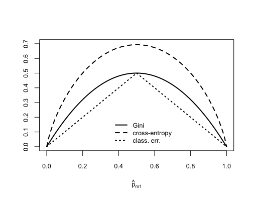
Figure 2: The Gini index, classification error, and cross-entropy in a simple classification setting with two classes. Question Majority approach: the number of red predictions is greater than the number of green predictions based on a 50% threshold, thus our prediction is RED.
Average approach: the average of the probabilities is less than the 50% threshold, thus our prediction is GREEN.
Applied Questions
-
library(tree)
fit <- tree(Sales ~ ., data = Carseats, subset = train)
plot(fit)
text(fit, pretty = 0)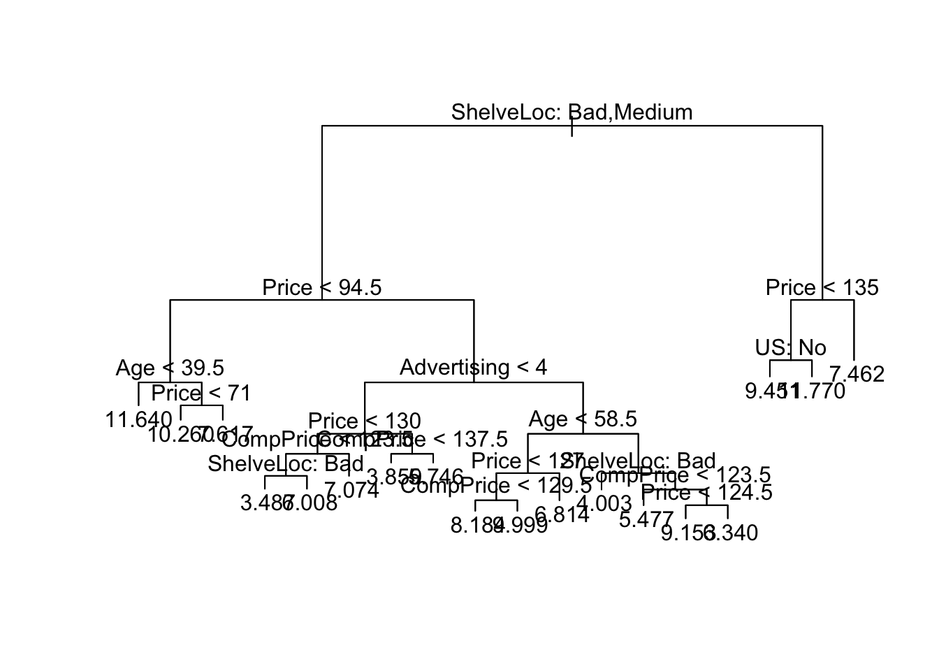
pred <- predict(fit, newdata = Carseats[!train, ])
(test.mse <- mean((Carseats$Sales[!train] - pred)^2))
[1] 4.922039The test MSE is about 4.92. Unfortunately, the plot doesn’t look too nice. Let’s try our luck with fitting function
rpart()from libraryrpartand plotting functionrpart.plot()from libraryrpart.plot(lots of libraries, I know).library(rpart) library(rpart.plot) fit.rpart <- rpart(Sales ~ ., data = Carseats, subset = train) rpart.plot(fit.rpart)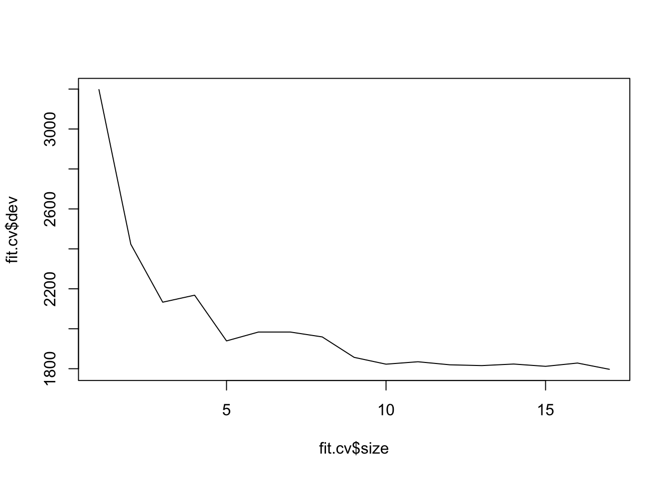
Much better! We see that
ShelveLocseems to be the most important predictor of sales (split at the top level), thenprice.set.seed(123) fit <- tree(Sales ~ ., data = Carseats) fit.cv <- cv.tree(fit, FUN = prune.tree) fit.cv$size [1] 17 16 15 14 13 12 11 10 9 8 7 6 5 4 3 2 1 $dev [1] 1967.759 1974.584 1988.813 2000.033 1972.183 1951.005 1961.298 1956.632 [9] 1928.169 1935.336 1915.630 1910.497 1876.414 2079.084 2122.798 2411.275 [17] 3199.248 $k [1] -Inf 32.78204 33.43341 34.30000 37.83019 38.65535 40.44960 [8] 41.83218 51.05171 70.52963 76.20847 76.57441 106.90014 145.33849 [15] 162.67977 334.36974 797.19286 $method [1] "deviance" attr(,"class") [1] "prune" "tree.sequence"plot(fit.cv$size, fit.cv$dev, type = "l")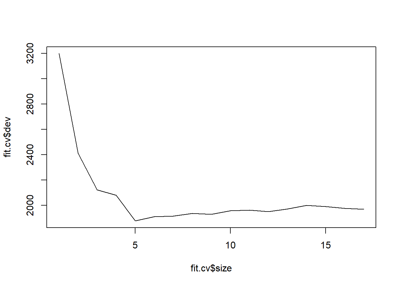
(index.min <- which.min(fit.cv$dev))[1] 13(size.min <- fit.cv$size[index.min])[1] 5plot(fit.cv$k, fit.cv$dev, type = "l")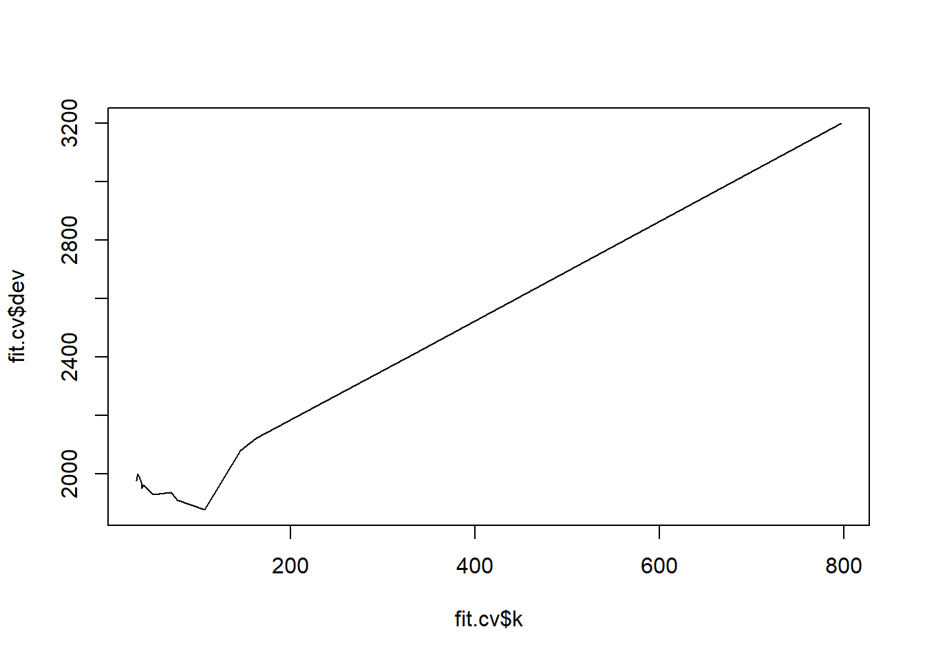
The model with the lowest CV error is the tree with 5 leaves. It has a cost-complexity tuning parameter of 106.9. Note the package calls the error “dev” for “deviance”, but this is equivalent to using the MSE.
library(randomForest)randomForest 4.7-1.2Type rfNews() to see new features/changes/bug fixes.set.seed(123) bag.sales <- randomForest(Sales ~ ., data = Carseats, subset = train, mtry = (ncol(Carseats) - 1), importance = TRUE ) pred <- predict(bag.sales, newdata = Carseats[!train, ]) (test.mse <- mean((Carseats$Sales[!train] - pred)^2))[1] 2.652066importance(bag.sales)%IncMSE IncNodePurity CompPrice 27.42854862 170.440734 Income 6.56405959 91.312337 Advertising 12.85200538 100.645018 Population -2.04530513 59.661563 Price 58.76321243 504.436464 ShelveLoc 46.41245711 364.580688 Age 15.71122036 156.907404 Education -0.48769025 42.691633 Urban 0.08928404 9.762364 US 4.29506266 17.020419The test error rate is 2.65, which is lower than the non-bagged regression tree model.
PriceandShelveLocare the most important predictors.set.seed(123) rf.sales <- randomForest(Sales ~ ., data = Carseats, subset = train, importance = TRUE ) pred <- predict(rf.sales, newdata = Carseats[!train, ]) (test.mse <- mean((Carseats$Sales[!train] - pred)^2))[1] 3.025767importance(rf.sales)%IncMSE IncNodePurity CompPrice 13.865262 154.23523 Income 1.690171 125.21748 Advertising 8.323675 111.76694 Population -3.143677 100.12141 Price 37.650327 387.58115 ShelveLoc 34.985856 294.92334 Age 12.057578 171.39258 Education -1.886551 75.67822 Urban 0.478542 16.63811 US 4.326428 31.86351The test error rate is 3.03, which is lower than with the nonbagged regression tree model, but higher than the bagged regression tree model.
PriceandShelveLocpredictors are most important, but their effect is understated compared to bagging.set.seed(1) rfTestMSE <- rep(Inf, ncol(Carseats) - 1) for (i in 1:(ncol(Carseats) - 1)) { rf.sales <- randomForest(Sales ~ ., data = Carseats, subset = train, mtry = i, importance = TRUE ) pred <- predict(rf.sales, newdata = Carseats[!train, ]) rfTestMSE[i] <- mean((Carseats$Sales[!train] - pred)^2) } plot(1:(ncol(Carseats) - 1), rfTestMSE, type = "l")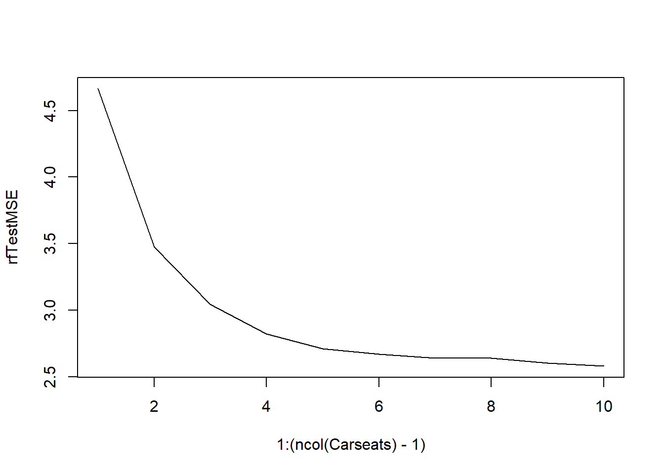
As expected, the test MSE shows a decreasing trend as the number of variables included in each random forest increases.
-
library(ISLR2) set.seed(1) train.set <- sample(1:nrow(OJ), 800) train <- 1:nrow(OJ) %in% train.setlibrary(tree) OJ.tree <- tree(Purchase ~ ., data = OJ, subset = train) summary(OJ.tree)Classification tree: tree(formula = Purchase ~ ., data = OJ, subset = train) Variables actually used in tree construction: [1] "LoyalCH" "PriceDiff" "SpecialCH" "ListPriceDiff" [5] "PctDiscMM" Number of terminal nodes: 9 Residual mean deviance: 0.7432 = 587.8 / 791 Misclassification error rate: 0.1588 = 127 / 800The training error rate is 0.1588 with 9 terminal nodes.
# you can type in the tree name "OJ.tree"
# here but it is easier to see in plot form
plot(OJ.tree)
text(OJ.tree)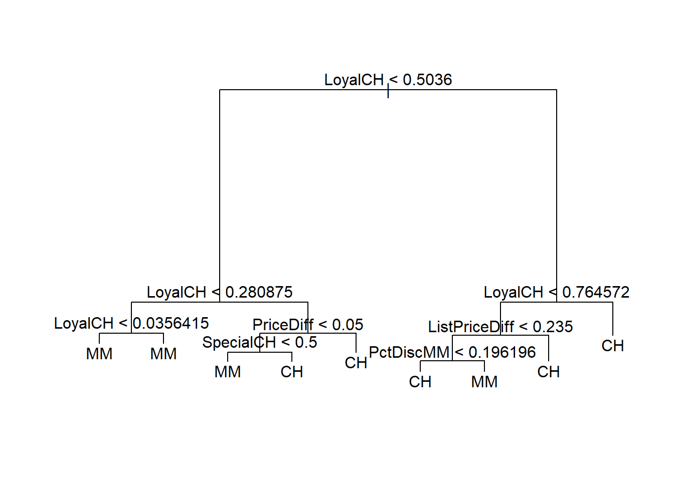
Consider the 4th leaf-node from the left: if 0.2809 < LoyalCH < 0.5036 and PriceDiff < 0.05 and SpecialCH > 0.5, then classify as CH.
See (c).
pred <- predict(OJ.tree, newdata = OJ[!train, ], type = "class")
table(pred = pred, true = OJ$Purchase[!train])
true pred CH MM CH 160 38 MM 8 64The test error rate is 0.1704.
set.seed(1) OJ.cv <- cv.tree(OJ.tree, FUN = prune.misclass)plot(OJ.cv$size, OJ.cv$dev, type = "l")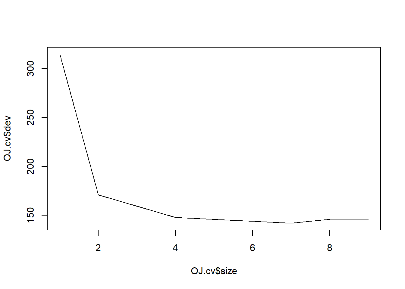
The optimal-sized tree has 7 leaves (aka terminal nodes).
See (g)
OJ.prune <- prune.misclass(OJ.tree, best = 7)table(fitted = predict(OJ.prune, type = "class"), true = OJ$Purchase[train])true fitted CH MM CH 441 86 MM 44 229table(fitted = predict(OJ.tree, type = "class"), true = OJ$Purchase[train])true fitted CH MM CH 450 92 MM 35 223The training error of the pruned tree is slightly higher than the original tree (0.1625 > 0.1588).
pred.prune <- predict(OJ.prune, newdata = OJ[!train, ], type = "class")
table(pred = pred.prune, true = OJ$Purchase[!train])
true pred CH MM CH 160 36 MM 8 66pred.tree <- predict(OJ.tree, newdata = OJ[!train, ], type = "class") table(pred = pred.tree, true = OJ$Purchase[!train])true pred CH MM CH 160 38 MM 8 64The test error of the pruned tree is slighlty lower than the original tree (0.1630 < 0.1704).
-
library(ISLR2)
myHitters <- Hitters[!is.na(Hitters$Salary), ]
myHitters$Salary <- log(myHitters$Salary)
train <- c(rep(TRUE, 200), rep(FALSE, nrow(myHitters) - 200))library(gbm)Loaded gbm 2.2.2This version of gbm is no longer under development. Consider transitioning to gbm3, https://github.com/gbm-developers/gbm3set.seed(1) lambda <- 10^seq(-5, -0.2, by = 0.05) trainMSE <- rep(Inf, length(lambda)) testMSE <- rep(Inf, length(lambda)) for (i in 1:length(lambda)) { fit <- gbm(Salary ~ ., distribution = "gaussian", data = myHitters[train, ], n.trees = 1000, shrinkage = lambda[i] ) pred.train <- predict(fit, n.trees = 1000) pred.test <- predict(fit, newdata = myHitters[!train, ], n.trees = 1000) trainMSE[i] <- mean((myHitters$Salary[train] - pred.train)^2) testMSE[i] <- mean((myHitters$Salary[!train] - pred.test)^2) } plot(lambda, trainMSE, type = "l")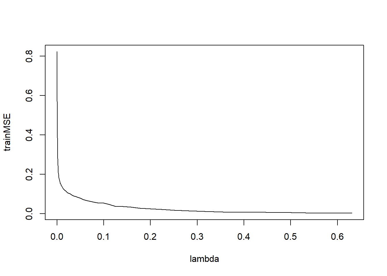
plot(lambda, testMSE, type = "l")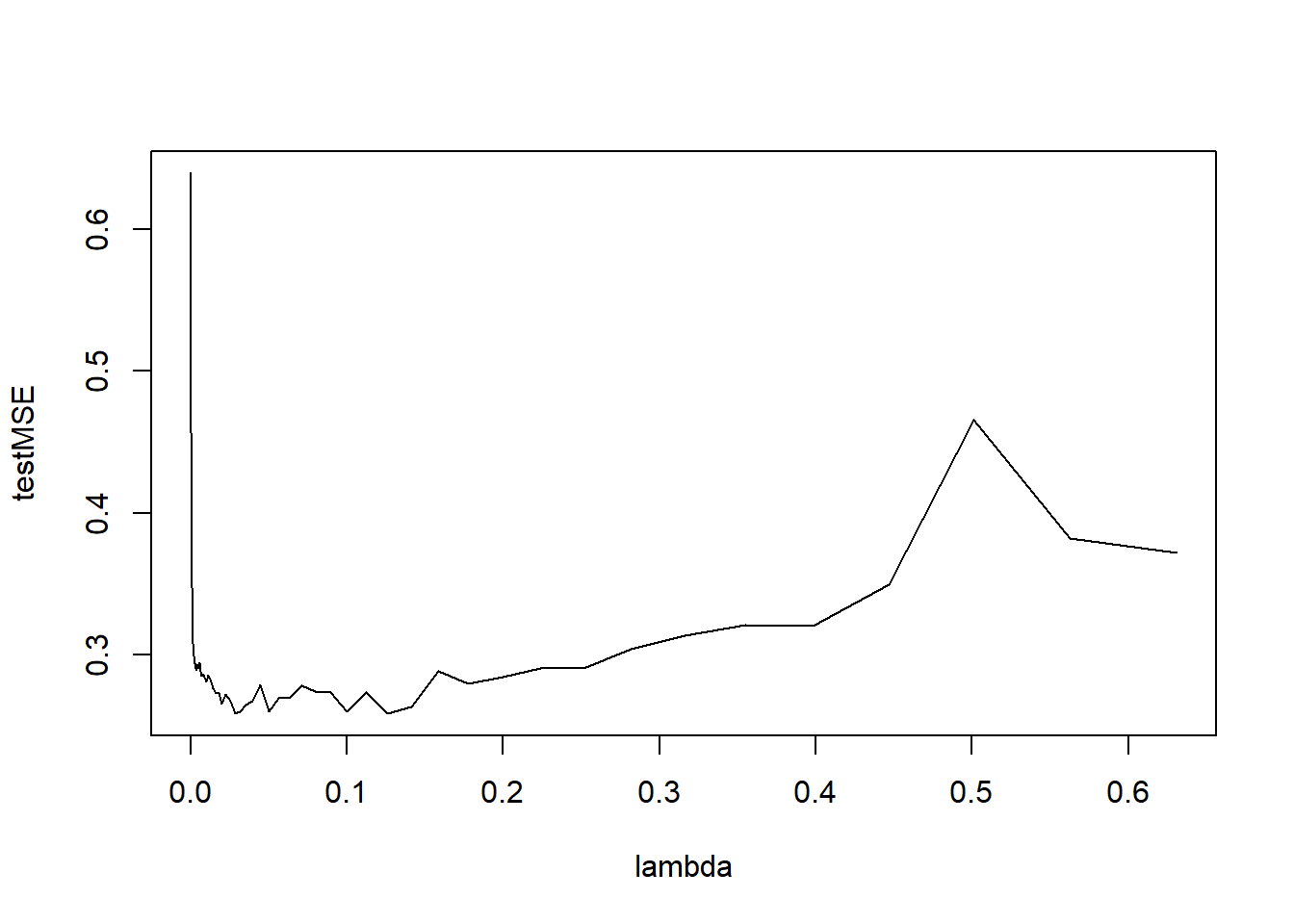
See (c)
library(MASS)Attaching package: 'MASS'The following object is masked from 'package:ISLR2': BostonmyHitters.lm <- stepAIC(lm(Salary ~ ., data = myHitters, subset = train), direction = "both" )Start: AIC=-187.65 Salary ~ AtBat + Hits + HmRun + Runs + RBI + Walks + Years + CAtBat + CHits + CHmRun + CRuns + CRBI + CWalks + League + Division + PutOuts + Assists + Errors + NewLeague Df Sum of Sq RSS AIC - CHmRun 1 0.0049 64.080 -189.64 - NewLeague 1 0.0129 64.088 -189.61 - CRBI 1 0.0220 64.097 -189.59 - Runs 1 0.0709 64.146 -189.43 - RBI 1 0.0751 64.150 -189.42 - CAtBat 1 0.0958 64.171 -189.35 - HmRun 1 0.1761 64.251 -189.10 - CHits 1 0.2560 64.331 -188.86 - League 1 0.2878 64.362 -188.76 - Errors 1 0.3521 64.427 -188.56 <none> 64.075 -187.65 - Division 1 0.8491 64.924 -187.02 - CRuns 1 0.8673 64.942 -186.97 - Assists 1 1.0963 65.171 -186.26 - CWalks 1 1.9086 65.983 -183.78 - Years 1 2.4861 66.561 -182.04 - AtBat 1 2.5729 66.648 -181.78 - Walks 1 2.8898 66.964 -180.83 - PutOuts 1 3.2769 67.352 -179.68 - Hits 1 4.3240 68.399 -176.59 Step: AIC=-189.64 Salary ~ AtBat + Hits + HmRun + Runs + RBI + Walks + Years + CAtBat + CHits + CRuns + CRBI + CWalks + League + Division + PutOuts + Assists + Errors + NewLeague Df Sum of Sq RSS AIC - NewLeague 1 0.0119 64.092 -191.60 - RBI 1 0.0875 64.167 -191.37 - Runs 1 0.0891 64.169 -191.36 - CAtBat 1 0.1110 64.191 -191.29 - HmRun 1 0.2377 64.317 -190.90 - League 1 0.2838 64.363 -190.75 - CRBI 1 0.3051 64.385 -190.69 - Errors 1 0.3510 64.431 -190.55 - CHits 1 0.5538 64.633 -189.92 <none> 64.080 -189.64 - Division 1 0.8580 64.938 -188.98 - Assists 1 1.0914 65.171 -188.26 + CHmRun 1 0.0049 64.075 -187.65 - CRuns 1 1.6078 65.687 -186.68 - CWalks 1 2.1324 66.212 -185.09 - Years 1 2.4813 66.561 -184.04 - AtBat 1 2.5702 66.650 -183.77 - Walks 1 2.9502 67.030 -182.64 - PutOuts 1 3.2741 67.354 -181.67 - Hits 1 4.4492 68.529 -178.21 Step: AIC=-191.6 Salary ~ AtBat + Hits + HmRun + Runs + RBI + Walks + Years + CAtBat + CHits + CRuns + CRBI + CWalks + League + Division + PutOuts + Assists + Errors Df Sum of Sq RSS AIC - Runs 1 0.0852 64.177 -193.34 - RBI 1 0.0870 64.179 -193.33 - CAtBat 1 0.1133 64.205 -193.25 - HmRun 1 0.2378 64.329 -192.86 - CRBI 1 0.3133 64.405 -192.63 - Errors 1 0.3435 64.435 -192.53 - CHits 1 0.5746 64.666 -191.82 <none> 64.092 -191.60 - League 1 0.6500 64.742 -191.58 - Division 1 0.8610 64.953 -190.93 - Assists 1 1.0989 65.190 -190.20 + NewLeague 1 0.0119 64.080 -189.64 + CHmRun 1 0.0040 64.088 -189.61 - CRuns 1 1.6393 65.731 -188.55 - CWalks 1 2.1279 66.219 -187.07 - Years 1 2.4904 66.582 -185.98 - AtBat 1 2.6070 66.699 -185.63 - Walks 1 2.9386 67.030 -184.63 - PutOuts 1 3.2764 67.368 -183.63 - Hits 1 4.4593 68.551 -180.15 Step: AIC=-193.34 Salary ~ AtBat + Hits + HmRun + RBI + Walks + Years + CAtBat + CHits + CRuns + CRBI + CWalks + League + Division + PutOuts + Assists + Errors Df Sum of Sq RSS AIC - RBI 1 0.0618 64.239 -195.14 - CAtBat 1 0.0870 64.264 -195.06 - HmRun 1 0.1634 64.340 -194.83 - Errors 1 0.3273 64.504 -194.32 - CRBI 1 0.4024 64.579 -194.09 - CHits 1 0.4926 64.669 -193.81 <none> 64.177 -193.34 - League 1 0.7004 64.877 -193.16 - Division 1 0.8457 65.022 -192.72 - Assists 1 1.1085 65.285 -191.91 + Runs 1 0.0852 64.092 -191.60 + CHmRun 1 0.0208 64.156 -191.40 + NewLeague 1 0.0080 64.169 -191.36 - CRuns 1 1.6598 65.837 -190.23 - CWalks 1 2.0465 66.223 -189.06 - Years 1 2.5245 66.701 -187.62 - AtBat 1 2.6071 66.784 -187.37 - Walks 1 3.0973 67.274 -185.91 - PutOuts 1 3.3751 67.552 -185.08 - Hits 1 5.2867 69.463 -179.50 Step: AIC=-195.14 Salary ~ AtBat + Hits + HmRun + Walks + Years + CAtBat + CHits + CRuns + CRBI + CWalks + League + Division + PutOuts + Assists + Errors Df Sum of Sq RSS AIC - HmRun 1 0.1074 64.346 -196.81 - CAtBat 1 0.1121 64.351 -196.79 - Errors 1 0.3404 64.579 -196.09 - CRBI 1 0.3411 64.580 -196.08 - CHits 1 0.5728 64.811 -195.37 <none> 64.239 -195.14 - League 1 0.6842 64.923 -195.02 - Division 1 0.8171 65.056 -194.62 - Assists 1 1.1172 65.356 -193.69 + RBI 1 0.0618 64.177 -193.34 + Runs 1 0.0600 64.179 -193.33 + CHmRun 1 0.0332 64.205 -193.25 + NewLeague 1 0.0082 64.230 -193.17 - CRuns 1 1.8768 66.115 -191.38 - CWalks 1 2.0449 66.283 -190.88 - Years 1 2.5017 66.740 -189.50 - AtBat 1 2.8465 67.085 -188.47 - Walks 1 3.0732 67.312 -187.80 - PutOuts 1 3.4528 67.691 -186.67 - Hits 1 5.2334 69.472 -181.48 Step: AIC=-196.81 Salary ~ AtBat + Hits + Walks + Years + CAtBat + CHits + CRuns + CRBI + CWalks + League + Division + PutOuts + Assists + Errors Df Sum of Sq RSS AIC - CAtBat 1 0.1313 64.477 -198.40 - Errors 1 0.3031 64.649 -197.87 - CRBI 1 0.6032 64.949 -196.94 - League 1 0.6451 64.991 -196.81 <none> 64.346 -196.81 - CHits 1 0.7286 65.075 -196.56 - Division 1 0.8421 65.188 -196.21 - Assists 1 1.0108 65.357 -195.69 + HmRun 1 0.1074 64.239 -195.14 + CHmRun 1 0.0722 64.274 -195.03 + NewLeague 1 0.0108 64.335 -194.84 + Runs 1 0.0074 64.339 -194.83 + RBI 1 0.0058 64.340 -194.83 - CRuns 1 2.0625 66.408 -192.50 - CWalks 1 2.1395 66.485 -192.27 - Years 1 2.4855 66.831 -191.23 - AtBat 1 2.7484 67.094 -190.44 - Walks 1 3.1563 67.502 -189.23 - PutOuts 1 3.4623 67.808 -188.33 - Hits 1 5.3023 69.648 -182.97 Step: AIC=-198.4 Salary ~ AtBat + Hits + Walks + Years + CHits + CRuns + CRBI + CWalks + League + Division + PutOuts + Assists + Errors Df Sum of Sq RSS AIC - Errors 1 0.3400 64.817 -199.35 <none> 64.477 -198.40 - League 1 0.6931 65.170 -198.26 - CRBI 1 0.7669 65.244 -198.04 - Division 1 0.8264 65.304 -197.85 - CHits 1 1.0305 65.508 -197.23 + CAtBat 1 0.1313 64.346 -196.81 + HmRun 1 0.1266 64.351 -196.79 + CHmRun 1 0.1138 64.363 -196.75 - Assists 1 1.2204 65.698 -196.65 + NewLeague 1 0.0145 64.463 -196.45 + RBI 1 0.0038 64.473 -196.41 + Runs 1 0.0002 64.477 -196.40 - CRuns 1 1.9601 66.437 -194.41 - CWalks 1 2.0480 66.525 -194.15 - AtBat 1 2.7199 67.197 -192.14 - Walks 1 3.0259 67.503 -191.23 - PutOuts 1 3.3495 67.827 -190.27 - Years 1 3.9323 68.410 -188.56 - Hits 1 5.4618 69.939 -184.14 Step: AIC=-199.35 Salary ~ AtBat + Hits + Walks + Years + CHits + CRuns + CRBI + CWalks + League + Division + PutOuts + Assists Df Sum of Sq RSS AIC - League 1 0.6153 65.433 -199.46 <none> 64.817 -199.35 - CRBI 1 0.7184 65.536 -199.14 - Division 1 0.8639 65.681 -198.70 - Assists 1 0.9112 65.728 -198.56 + Errors 1 0.3400 64.477 -198.40 - CHits 1 1.0614 65.879 -198.10 + CAtBat 1 0.1683 64.649 -197.87 + CHmRun 1 0.1027 64.715 -197.67 + HmRun 1 0.0859 64.731 -197.61 + NewLeague 1 0.0062 64.811 -197.37 + RBI 1 0.0000 64.817 -197.35 + Runs 1 0.0000 64.817 -197.35 - CWalks 1 1.9827 66.800 -195.32 - CRuns 1 1.9910 66.808 -195.30 - AtBat 1 3.0871 67.904 -192.04 - Walks 1 3.1044 67.922 -191.99 - PutOuts 1 3.3522 68.169 -191.26 - Years 1 4.1178 68.935 -189.03 - Hits 1 5.9080 70.725 -183.90 Step: AIC=-199.46 Salary ~ AtBat + Hits + Walks + Years + CHits + CRuns + CRBI + CWalks + Division + PutOuts + Assists Df Sum of Sq RSS AIC - CRBI 1 0.6392 66.072 -199.51 <none> 65.433 -199.46 + League 1 0.6153 64.817 -199.35 - Division 1 0.8091 66.242 -199.00 - CHits 1 0.8163 66.249 -198.98 + NewLeague 1 0.3785 65.054 -198.62 - Assists 1 0.9543 66.387 -198.56 + Errors 1 0.2622 65.170 -198.26 + CAtBat 1 0.2134 65.219 -198.11 + CHmRun 1 0.0934 65.339 -197.75 + HmRun 1 0.0579 65.375 -197.64 + Runs 1 0.0075 65.425 -197.48 + RBI 1 0.0006 65.432 -197.46 - CRuns 1 1.7237 67.156 -196.26 - CWalks 1 1.8619 67.294 -195.85 - AtBat 1 3.2103 68.643 -191.88 - Walks 1 3.3974 68.830 -191.34 - PutOuts 1 3.4478 68.880 -191.19 - Years 1 3.8438 69.276 -190.04 - Hits 1 5.7897 71.222 -184.50 Step: AIC=-199.52 Salary ~ AtBat + Hits + Walks + Years + CHits + CRuns + CWalks + Division + PutOuts + Assists Df Sum of Sq RSS AIC - CHits 1 0.5086 66.580 -199.98 + CHmRun 1 0.7324 65.339 -199.74 - Assists 1 0.6552 66.727 -199.54 <none> 66.072 -199.51 + CRBI 1 0.6392 65.433 -199.46 + League 1 0.5361 65.536 -199.14 - Division 1 0.8042 66.876 -199.09 + CAtBat 1 0.3820 65.690 -198.68 + HmRun 1 0.3080 65.764 -198.45 + NewLeague 1 0.2843 65.787 -198.38 + Errors 1 0.2266 65.845 -198.20 + RBI 1 0.1568 65.915 -197.99 + Runs 1 0.0180 66.054 -197.57 - CWalks 1 1.5544 67.626 -196.87 - CRuns 1 1.8017 67.873 -196.13 - AtBat 1 2.9686 69.040 -192.72 - Walks 1 3.3606 69.432 -191.59 - PutOuts 1 3.5426 69.614 -191.07 - Years 1 4.1936 70.265 -189.21 - Hits 1 5.6890 71.761 -185.00 Step: AIC=-199.98 Salary ~ AtBat + Hits + Walks + Years + CRuns + CWalks + Division + PutOuts + Assists Df Sum of Sq RSS AIC + CHmRun 1 0.9592 65.621 -200.88 - Assists 1 0.4404 67.021 -200.66 <none> 66.580 -199.98 + CHits 1 0.5086 66.072 -199.51 + HmRun 1 0.4522 66.128 -199.34 + League 1 0.3603 66.220 -199.07 + CRBI 1 0.3316 66.249 -198.98 + Errors 1 0.2653 66.315 -198.78 - Division 1 1.1221 67.703 -198.64 + RBI 1 0.1526 66.428 -198.44 - CWalks 1 1.1927 67.773 -198.43 + NewLeague 1 0.1262 66.454 -198.36 + CAtBat 1 0.0864 66.494 -198.24 + Runs 1 0.0508 66.530 -198.13 - CRuns 1 2.4724 69.053 -194.69 - AtBat 1 2.6054 69.186 -194.30 - PutOuts 1 3.1307 69.711 -192.79 - Walks 1 3.7084 70.289 -191.14 - Years 1 3.7734 70.354 -190.96 - Hits 1 5.2100 71.790 -186.91 Step: AIC=-200.88 Salary ~ AtBat + Hits + Walks + Years + CRuns + CWalks + Division + PutOuts + Assists + CHmRun Df Sum of Sq RSS AIC <none> 65.621 -200.88 + League 1 0.4883 65.133 -200.38 - Assists 1 0.8610 66.482 -200.28 - CHmRun 1 0.9592 66.580 -199.98 + Errors 1 0.3065 65.315 -199.82 - Division 1 1.0239 66.645 -199.79 + CHits 1 0.2818 65.339 -199.74 + NewLeague 1 0.2366 65.385 -199.61 + CRBI 1 0.1907 65.430 -199.47 + CAtBat 1 0.0667 65.555 -199.09 + HmRun 1 0.0422 65.579 -199.01 + Runs 1 0.0383 65.583 -199.00 + RBI 1 0.0157 65.606 -198.93 - CWalks 1 1.5295 67.151 -198.28 - CRuns 1 1.6423 67.263 -197.94 - AtBat 1 3.0894 68.711 -193.68 - PutOuts 1 3.1887 68.810 -193.39 - Years 1 3.7086 69.330 -191.89 - Walks 1 3.7259 69.347 -191.84 - Hits 1 5.6581 71.279 -186.34set.seed(1) require(glmnet)Loading required package: glmnetLoading required package: MatrixLoaded glmnet 4.1-8myHitters.cv <- cv.glmnet(model.matrix(Salary ~ ., data = myHitters[train, ]), myHitters$Salary[train], alpha = 1 ) myHitters.lasso <- glmnet(model.matrix(Salary ~ ., data = myHitters[train, ]), myHitters$Salary[train], alpha = 1 ) myHitters.pred.lasso <- predict(myHitters.lasso, type = "response", newx = model.matrix(Salary ~ ., data = myHitters[!train, ] ) ) myHitters.pred.lm <- predict(myHitters.lm, newdata = myHitters[!train, ]) mean((myHitters.pred.lasso - myHitters$Salary[!train])^2)[1] 0.4755605mean((myHitters.pred.lm - myHitters$Salary[!train])^2)[1] 0.4931775The MSE’s of the linear model and the lasso model seem to be higher than the MSE of the boosted model except for larger values of \lambda.
summary(fit)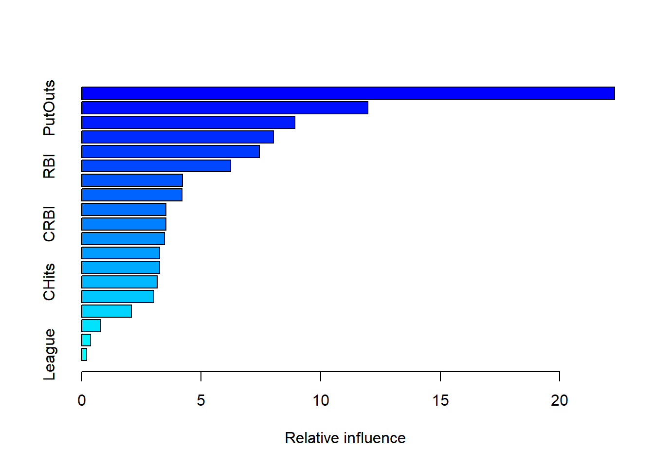
CAtBat and PutOuts appear to be the most important outputs.
library(randomForest)
set.seed(1)
myHitters.bag <- randomForest(Salary ~ .,
  data = myHitters, subset = train,
  mtry = (ncol(myHitters) - 1), importance = TRUE
)
pred <- predict(myHitters.bag, newdata = myHitters[!train, ])
mean((myHitters$Salary[!train] - pred)^2)
[1] 0.2301184The test MSE is 0.229, which is lower than the minimum test MSE from the boosted model.