Introduction to Statistical Learning

Disclaimer

Some of the figures in this presentation are taken from “An Introduction to Statistical Learning, with applications in R” (Springer, 2013) with permission from the authors: G. James, D. Witten, T. Hastie and R. Tibshirani.

Overview

• Data Science vs Actuarial Science
• Overview of Statistical Learning
• Model Accuracy in Regression Problems
• Classification Problems

Reading

James et al. (2021), Chapters 1 and 2

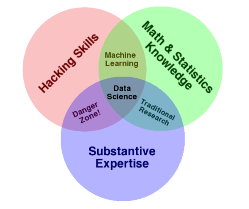
Data Science vs Actuarial Science

Data Science Skills

Source: THE DATA SCIENCE VENN DIAGRAM, Drew Conway Data Consulting

Actuaries use data for good

Source: Actuaries Institute

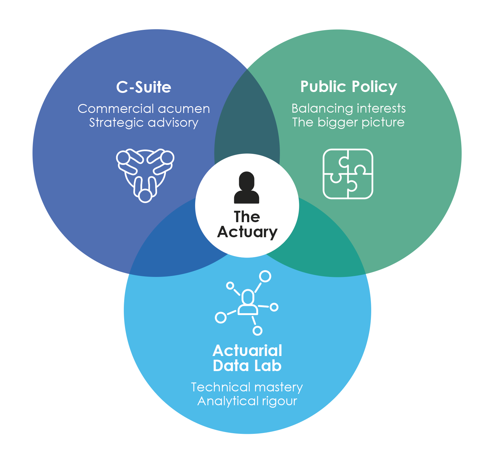
Do data better with an Actuary

Source: dodatabetter.com.au (Actuaries Institute)

Overview of Statistical Learning

Statistical Learning / Predictive Analytics

• A vast set of tools for understanding data.
• Other names used to refer to similar tools (sometimes with a slightly different viewpoint) - machine learning, predictive analytics.
• Techniques making significant impact to actuarial work especially in the insurance industry.
• Historically - started with classical linear regression techniques.
• Contemporary extensions included:
  • better methods to apply regression ideas
  • non-linear models
  • unsupervised problems
• Facilitated by powerful computation techniques and accessible software such as R.

What is statistical (machine) learning?

What is statistical (machine) learning?

Goals of statistical (machine) learning

Prediction

• Predict outcomes of Y given X
• The “meaning” or “interpretation” of f(\cdot) is not the focus, we just want accurate predictions
• Models can be very complex

Inference

• Understand how X affects Y
• Which predictors should we add, and what is their individual contribution to explain Y? How are they related?
• Models tend to be simpler

The Two Cultures

	Statistical Learning	Machine Learning
Origin	Statistics	Computer Science
f(X)	Model	Algorithm
Emphasis	Interpretability, precision and uncertainty	Large scale application and prediction accuracy
Jargon	Parameters, estimation	Weights, learning
Confidence interval	Uncertainty of parameters	No notion of uncertainty
Assumptions	Explicit a priori assumption	No prior assumption, we learn from the data

See Breiman (2001)

What is statistical (machine) learning?

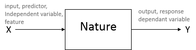
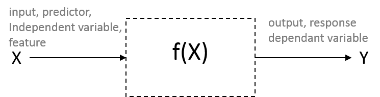
Many models have the following general form:

Y = f(X) + \epsilon

• Y is the output (or “outcome”, “response”, “dependent variable”)
• X:=(X_1, X_2, \ldots, X_p) are the inputs (or “predictors”, “features”, “independent variables”)
• \epsilon is the error (or “noise”) which reflects that a model is (almost) never perfect, because of random chance, measurement error and other discrepancies

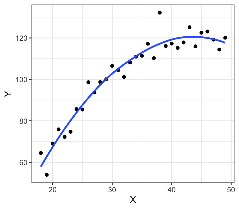
\Rightarrow Our objective is to find an appropriate f for the problem at hand. If Y is quantitative, we call this a regression problem, which can be non-trivial.

• What Xs should we choose?
• Do we want to predict reality (prediction) or explain reality (inference)?
• What’s signal and what’s noise?

How to estimate f?

Parametric

• Make an assumption about the shape of f
• Problem reduced down to estimating a few parameters
  • Works fine with limited data, provided assumption is reasonable
• Strong assumption: tends to miss some signal

Non-parametric

• Make no assumption about f’s shape
• Involves estimating a lot of “parameters”
  • Typically needs lots of data
• Weak or no assumption: tends to mistake noise for signal
• Be particularly careful about the risk of overfitting

Example: Linear model fit on income data

Using Education and Seniority to explain Income:

• Linear model fitted
• Does a pretty decent job of fitting the data, by the looks of it, but doesn’t capture everything

Example: “perfect” fit on income data

• Non-parametric spline fit
• Fits the data perfectly: this is indicative of overfitting

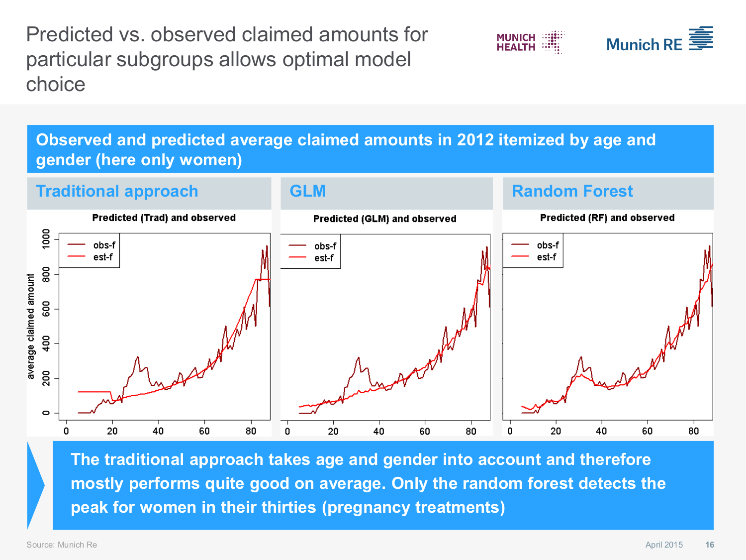
Actuarial Application: Health Insurance model choice

Tradeoff between interpretability and flexibility

• We will cover a number of different methods in this course
• They each have their own (relative) combinations of interpretability and flexibility:

Discussion Question

Suppose you are interested in prediction. Everything else being equal, which types of methods would you prefer?

Supervised vs unsupervised learning

Supervised

• There is a response (y_i) for each set of predictors (x_{ij})
• e.g. Linear regression, logistic regression
• Can find a f that “boil down” predictors into a response

Unsupervised

• No y_i, just sets of x_{ij}
• e.g. Cluster analysis
• Can only find associations between predictors

Cluster analysis is a form of unsupervised learning

• The idea is to identify clusters: groups of points that are “similar”.
  
• Here, for illustration we have provided the real groups (in different colours), but in reality the actual grouping is not known in an unsupervised problem. Hence, “we are in some sense working blind” (James et al., 2021).
• The example of the right would be more difficult to cluster properly.

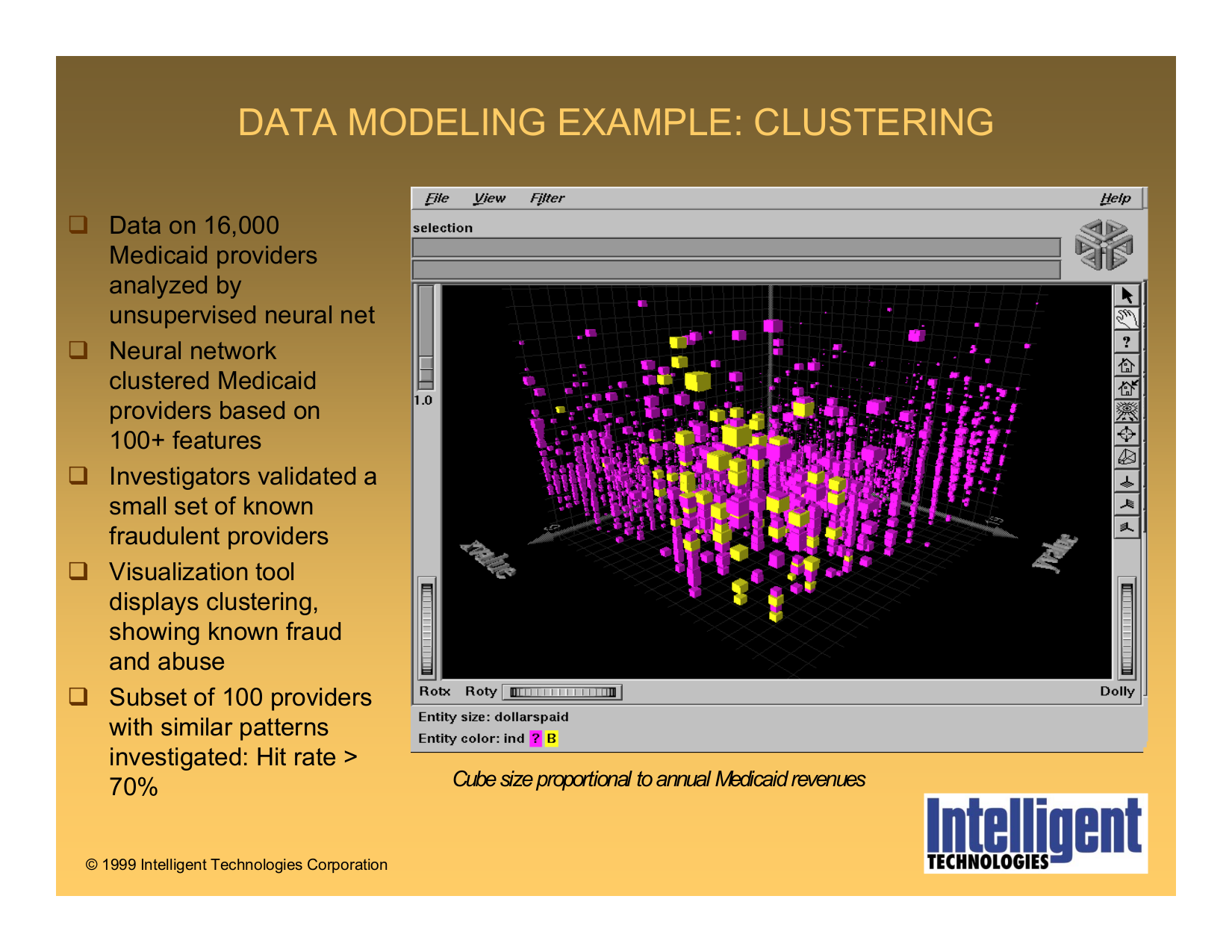
Actuarial Application: predict claim fraud and abuse

A note re Regression vs Classification problems

Regression

• Y is quantitative
• Examples: Sales prediction, claim size prediction, stock price modelling

Classification

• Y is qualitative (or “categorial”, or “discrete”)
• Examples: fraud detection, face recognition, death

Model Accuracy in Regression Problems

Assessing Model Accuracy: MSE

• There are often a wide range of possible statistical learning methods that can be applied to a problem.
• There is no single method that dominates over all others in all data sets.
• How do we assess the accuracy or “quality of fit” of our model?
  • Mean Squared Error \text{MSE} = \frac{1}{n} \sum_{i=1}^{n}(y_i-\hat{f}(x_i))^2
  • This will be small if predicted responses are close to actual responses.
  • If the MSE is computed using the data used to fit the model (which is called the training data), this is more accurately referred to as the training MSE.

Discussion question

Do you see potential problems with using the training MSE to evaluate a model?

Example: which model is best?

• On the left plot, the true function f() is the black line, used to generate a sample of (X,Y), displayed as a scatterplot. Three different fitted models are illustrated as the blue, green and orange lines. On the right plot, training MSE (gray) and test MSE (red) of the respetive models are displayed.

Examples: Assessing model accuracy

The following are the training and test errors for three different problems:

Bias-Variance Tradeoff

Consider x_0, the predictor(s) of an observation that is not in the training data. The expected test MSE at x_0 can be written as:

\mathbb{E}\bigl(y_0 - \hat{f}(x_0)\bigr)^2 = \text{Var}(\hat{f}(x_0)) + [\text{Bias}(\hat{f}(x_0))]^2 + \text{Var}(\epsilon)

• \text{Var}(\hat{f}(x_0)): the variability in the prediction (think of this as “by how much \hat{f} would change if a different training set was used”)
• [\text{Bias}(\hat{f}(x_0))]^2: the average (or “systematic”) error of the model
• \text{Var}(\epsilon): the irreducible error

In machine learning problems, there is usually a tradeoff between Bias and Variance (i.e., you can’t improve both simultaneously). In general, “as we use more flexible methods, the variance will increase and the bias will decrease” (James et al., 2021).

Examples: Bias-variance tradeoff

The following are the Bias-Variance tradeoff for three different problems:

Classification Problems

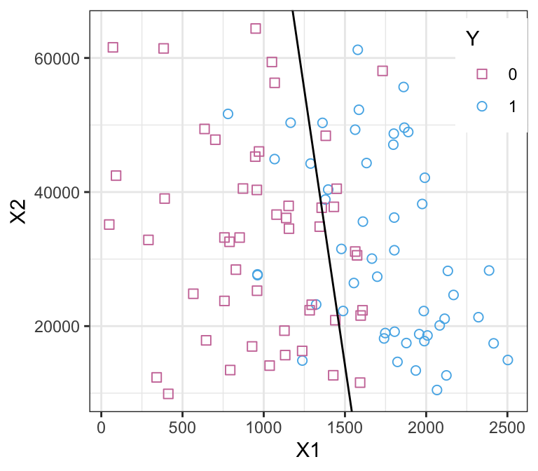
What is Classification?

• When we want to predict the category of a qualitative variable Y, we are facing a “classification problem”.
• Objective: assign a data point into a category (Y_i value) based on its predictors (X_{i,j} values).
• Training Error rate: proportion of mistakes made (i.e., our prediction is wrong) when applying the estimate \hat{f} to the training data: \frac{1}{n} \sum_{i=1}^n \mathbb{I}(y_i \neq \hat{y}_i)
• Test Error rate: proportion of mistakes made when applying the estimate \hat{f} to a test data (i.e., observations the model was not trained on): \text{Ave}\left(\mathbb{I}(y_0 \neq \hat{y}_0)\right)

Bayes’ Classifier

• This is the ideal classifier, but is not computable in practice. You can view it as the “gold standard against which to compare other methods” (James et al., 2021).
• It simply assigns a test observation (with predictor x_0) to the class \color{magenta}{j} which maximises \mathbb{P}(Y={\color{magenta}{j}}|X=x_0).
• In the case of two classes, this would be the class \color{magenta}{j} for which \mathbb{P}(Y={\color{magenta}{j}}|X=x_0) > 0.5.
• This classifier minimises the test error rate, but it is not computable in practical problems because in real life we don’t know the theoretical conditional probabilities \mathbb{P}[Y=y|X=x].
• A simple alternative is the K-nearest neighbours (KNN) classifier.

K-nearest neighbours - illustration

K-nearest neighbours

• Consider a new observation x_0 (for which we want to predict the “Y” class).
• Call \mathcal{N}_0 the set of x_0’s K-nearest (training) observations.
• Classify x_0 to the class \color{magenta}{j} that maximises \frac{1}{K}\sum_{i\in\mathcal{N}_0} \mathbb{I}(y_i={\color{magenta}{j}}),
• This makes sense because the above approximates \mathbb{P}(Y={\color{magenta}{j}}|X=x_0).
• In words: a new observation’s “Y class” is set to the majority “Y class” of its neighbours.
• A smart choice of K is crucial:
  • K too high: less variance but more bias. Fit is closer to a “global average” (you are not capturing all the meaningful signal).
  • K too low: less bias but more variance. Fit mistakes some noise for signal (you are overfitting).

K-nearest neighbours example, K=10

(purple is the Bayes boundary, black is the KNN boundary with K=10)

K-nearest neighbours example, K=1, K=100

References

James, G., Witten, D., Hastie, T., & Tibshirani, R. (2021). An Introduction to Statistical Learning: with Applications in R. Springer.