Lab 6: Cross-validation & Regularisation

Questions

Conceptual Questions

\star Solution (ISLR2, Q5.3) Consider k-fold cross-validation.
1. Explain how k-fold cross-validation is implemented.
2. What are the advantages and disadvantages of k-fold cross-validation relative to:
  - The validation set approach?
  - LOOCV?
\star Solution (ISLR2, Q6.2) For parts (a) through (c), indicate which of i. through iv. is correct. Justify your answer.
1. The lasso, relative to least squares, is:
  1. More flexible and hence will give improved prediction accuracy when its increase in bias is less than its decrease in variance.
  2. More flexible and hence will give improved prediction accuracy when its increase in variance is less than its decrease in bias.
  3. Less flexible and hence will give improved prediction accuracy when its increase in bias is less than its decrease in variance.
  4. Less flexible and hence will give improved prediction accuracy when its increase in variance is less than its decrease in bias.
2. Repeat (a) for ridge regression relative to least squares.
3. Repeat (a) for non-linear methods relative to least squares.
\star Solution (ISLR2, Q6.3) Suppose we estimate the regression coefficients in a linear regression model by minimising \sum_{i=1}^n \Bigl( y_i - \beta_0 - \sum_{j=1}^p\beta_ix_{ij} \Bigr)^2 \text{ subject to } \sum_{j=1}^p |\beta_j| \leq s for a particular value of s. For parts (a) through (e), indicate which of i. through v. is the (only) correct choice. Justify your answer.
1. As we increase s from 0, the training RSS will:
  1. Increase initially, and then eventually start decreasing in an inverted U shape.
  2. Decrease initially, and then eventually start increasing in a U shape.
  3. Steadily increase.
  4. Steadily decrease.
  5. Remain constant.
2. Repeat (a) for test RSS.
3. Repeat (a) for variance of parameters’ estimates.
4. Repeat (a) for (squared) bias of parameters’ estimates.
5. Repeat (a) for the irreducible error.
Solution (ISLR2, Q6.5, modified) It is well-known that ridge regression tends to give similar coefficient values to correlated variables, whereas the lasso may give quite different coefficient values to correlated variables. We will now explore this property in a very simple setting.
Suppose that n=2, p= 2, x_{11} = x_{12}, x_{21} = x_{22}. Furthermore, suppose that y_1+y_2 = 0 and x_{11}+x_{21} = 0 and x_{12}+x_{22} = 0, so that the estimate for the intercept in a least squares, ridge regression, or lasso model is zero: \hat{\beta}_0 = 0.
1. Write out the ridge regression optimisation problem in this setting.
2. In this setting, find the ridge coefficient estimates for \beta_1, \beta_2. In particular, show that they satisfy \hat{\beta}_1 = \hat{\beta}_2.
3. Write out the lasso optimisation problem in this setting.
4. Argue that in this setting, the lasso coefficients have several solutions, for which \hat{\beta}_1 \neq \hat{\beta}_2. Describe these solutions. Hint: use the alternative formulation of the lasso constraint, in terms of a “budget” s.
Solution Optional: Show that the LOOCV mean squared error for linear models is: CV_{(n)} = \frac{1}{n} \sum_{i=1}^n \left(\frac{y_i-\hat{y}_i}{1-h_i}\right)^2 Take note of the Sherman-Morrison formula: (A+uv^T)^{-1} = A^{-1} - \frac{A^{-1}uv^T A^{-1}}{1 + v^TA^{-1}u} where A is an invertible square matrix, and u, v are column vectors.

Applied Questions

\star Solution (ISLR2, Q5.5) In Chapter 4, we used logistic regression to predict the probability of default using income and balance on the Default data set. We will now estimate the test error of this logistic regression model using the validation set approach. Do not forget to set a random seed before beginning your analysis.
1. Fit a logistic regression model that uses income and balance to predict default. What is the error rate of that model, on the entire dataset (i.e., training error rate)?
2. Using the validation set approach, estimate the test error of this model. In order to do this, you must perform the following steps:
  1. Split the sample set into a training set and a validation set.
  2. Fit a multiple logistic regression model using only the training observations.
  3. Obtain a prediction of default status for each individual in the validation set by computing the posterior probability of default for that individual, and classifying the individual to the default category if the posterior probability is greater than 0.5.
  4. Compute the validation set error, which is the fraction of the observations in the validation set that are misclassified.
3. Repeat the process in (b) three times, using three different splits of the observations into a training set and a validation set. Comment on the results obtained.
4. Now consider a logistic regression model that predicts the probability of default using income, balance, and a dummy variable for student. Estimate the test error for this model using the validation set approach. Comment on whether or not including a dummy variable for student leads to a reduction in the test error rate.
Solution (ISLR2, Q5.7) In Sections 5.3.2 and 5.3.3, we saw that the cv.glm() function can be used in order to compute the LOOCV test error estimate. Alternatively, one could compute those quantities using just the glm() and predict.glm() functions, and a for loop. You will now take this approach in order to compute the LOOCV error for a simple logistic regression model on the Weekly data set. Recall that in the context of classification problems, the LOOCV error is given in (5.4).
1. Fit a logistic regression model that predicts Direction using Lag1 and Lag2.
2. Fit a logistic regression model that predicts Direction using Lag1 and Lag2 using all but the first observation.
3. Use the model from (b) to predict the direction of the first observation. You can do this by predicting that the first observation will go up if \mathbb{P}(\texttt{Direction = "Up"} | \texttt{Lag1}, \texttt{Lag2}) > 0.5. Was this observation correctly classified?
4. Write a for loop from i=1 to i=n, where n is the number of observations in the data set, that performs each of the following steps:
  1. Fit a logistic regression model using all but the ith observation to predict Direction using Lag1 and Lag2.
  2. Compute the posterior probability of the market moving up for the ith observation.
  3. Use the posterior probability for the ith observation in order to predict whether or not the market moves up.
  4. Determine whether or not an error was made in predicting the direction for the ith observation. If an error was made, then indicate this as a 1, and otherwise indicate it as a 0.
5. Take the average of the n numbers obtained in d.-iv. in order to obtain the LOOCV estimate for the test error. Comment on the results.
\star Solution (ISLR2, Q5.8) We will now perform cross-validation on a simulated data set.
1. Generate a simulated data set as follows:
```
set.seed(1)
x <- rnorm(100)
y <- x - 2 * x^2 + rnorm(100)
```
  In this data set, what is n and what is p? Write out the model used to generate the data in equation form.
2. Create a scatterplot of X against Y. Comment on what you find.
3. Set a random seed, and then compute the LOOCV errors that result from fitting the following four models using least squares:
  1. Y = \beta_0 + \beta_1 X + \epsilon
  2. Y = \beta_0 + \beta_1 X + \beta_2X^2+ \epsilon
  3. Y = \beta_0 + \beta_1 X + \beta_2X^2+ \beta_3X^3 + \epsilon
  4. Y = \beta_0 + \beta_1 X + \beta_2X^2+ \beta_3X^3 + \beta_4X^4 + \epsilon
  Note you may find it helpful to use the data.frame() function to create a single data set containing both X and Y .
4. Repeat (c) using another random seed, and report your results. Are your results the same as what you got in (c)? Why?
5. Which of the models in (c) had the smallest LOOCV error? Is this what you expected? Explain your answer.
6. Comment on the statistical significance of the coefficient estimates that results from fitting each of the models in (c) using least squares. Do these results agree with the conclusions drawn based on the cross-validation results?
\star Solution (ISLR2, Q6.9, modified) Refer to the data set College from package ISLR2. In this exercise, we will predict the graduation rate Grad.Rate (last variable in the data set) using all the other variables as predictors.
1. Split the data set into a training set (2/3 of the data) and a test set (1/3).
2. Fit a linear model using least squares on the training set, and report both the “training error” and “test error” obtained.
3. Fit a ridge regression model on the training set. Find the MSE on the test set with the arbitrary choice \lambda=10. Then, use function cv.glm to chose the “best” \lambda by cross-validation. Report the new test MSE obtained, and briefly discuss the result.
4. Fit a lasso model on the training set, with \lambda chosen by cross-validation. Report the test MSE obtained, along with the number of non-zero coefficient estimates.
5. Comment on the results obtained. How accurately can we predict Grad.Rate? Is there much difference among the test errors resulting from these three approaches (Linear Regression, Ridge and Lasso Regressions)?
Solution (ISLR2, Q6.10, modified) We have seen that as the number of features used in a model increases, the training error will necessarily decrease, but the test error may not. We will now explore this in a simulated data set.
1. Generate a data set with p = 20 features, n = 1,\!000 observations, and an associated quantitative response vector generated according to the model Y = X \beta + \epsilon where \beta has some elements that are exactly equal to zero.
2. Split your data set into a training set containing 100 observations and a test set containing 900 observations.
3. Perform best subset selection on the training set, and plot the training set MSE associated with the best model of each size.
4. Plot the test set MSE associated with the best model of each size.
5. For which model size does the test set MSE take on its minimum value? Comment on your results. If it takes on its minimum value for a model containing only an intercept or a model containing all of the features, then play around with the way that you are generating the data in (a) until you come up with a scenario in which the test set MSE is minimized for an intermediate model size.
6. How does the model at which the test set MSE is minimized compare to the true model used to generate the data? Comment on the coefficient values.
7. Lastly, try Lasso Regression on your entire simulated dataset, and comment on its performance.

Solutions

Conceptual Questions

Question Refer to Module 5 lecture slides and Chapter 5 of the book for this question.
Question
1. 1. Incorrect: lasso is less flexible than least squares (as some coefficients are shrunk to 0).
  2. Incorrect again.
  3. Correct! If lasso trades a relatively small increase in bias for a more subtantial reduction in parameters estimates’ variance, lasso can lead to better predictions.
  4. Incorrect, because we expect a decrease in parameters estimates’ variance (at the cost of increased bias).
2. The same answers as for lasso hold. Indeed, ridge is still a “less flexible” method than regular least squares regression: we restrict the size of the parameter estimates. This is a constraint (or “inflexibility”) that regular least squares does not have.
3. 1. Incorrect, as more flexibility means lower bias but higher variance.
  2. Correct! It is more flexible since least squares only does a linear fit.
  3. Incorrect, non-linear methods are more flexible.
  4. Incorrect again.
Question

The central concept here is that increasing s increases the model’s flexibility (in the limit of s=\infty, we fall back on regular least squares regression). And with more flexibility, we expect the model’s fit on the training data to be better (but, on test data, a model that is too flexible won’t perform well, due to overfitting).
1. iii.
2. ii. Initially, it will decrease as the model fits more signal. However, at some point, the model will start overfitting the training data, which means the performance on the test data will worsen.
3. iii. As the model becomes more flexible, the variance will increase.
4. iv. As the model becomes more flexible, its bias will decrease.
5. v. Irreducible error is irreducible (it is unaffected by the specific choice of model).
Question
1. Because x_{11}=x_{12}, let’s just call those values “x_1”. Likewise, let “x_2” denote the value x_{21}=x_{22}. Then, we are minimising for \beta_1, \beta_2 in: \sum_{i=1}^2 (y_i - (\beta_1 + \beta_2)x_{i})^2 + \lambda (\beta_1^2 + \beta_2^2).
2. Call “\text{rdg}” the quantity above, which we want to minimise. We take its partial derivatives with respect to \beta_1 and \beta_2. This gives us two equations, which we set to 0 and solve.
  
  \begin{align*} \frac{\partial \, \text{rdg}}{\partial \beta_j} = \sum_i 2(y_i - (\beta_1 + \beta_2)x_{i})(-x_i) + 2 \lambda \beta_j = 0 \end{align*} \begin{align*} \text{Equation 1:} \, \sum_i -x_i y_i + x_i^2 (\beta_1 + \beta_2) + \lambda \beta_1 & = 0 \\ \text{Equation 2:} \, \sum_i -x_i y_i + x_i^2 (\beta_1 + \beta_2) + \lambda \beta_2 & = 0 \\ \implies \lambda \beta_1 - \lambda \beta_2 = 0 \implies \beta_1 = \beta_2. \end{align*}
  
  Hence, we indeed have that the estimates will satify \beta_1=\beta_2. To find the final solution, just replace \beta_2 by \beta_1 in one of these equations, and solve: \begin{align*} 2 \beta_1 \sum_i x_i^2 + \lambda \beta_1 & = \sum_i x_i y_i \\ \beta_1 & = \frac{\sum_i x_i y_i}{2 \sum x_i^2 + \lambda}. \end{align*}
3. We are minimising for \beta_1, \beta_2 in: \sum_{i=1}^2 (y_i - (\beta_1 + \beta_2)x_{i})^2 + \lambda (|\beta_1| + |\beta_2|).
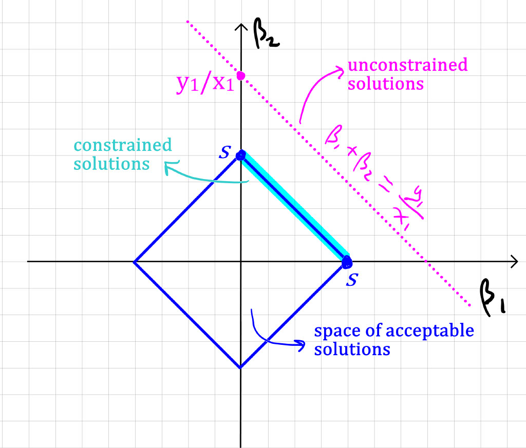
4. Unfortunately, we can’t differentiate the absolute value function f(t)=|t|, so we can’t rely on the approach from part b. Instead, we need to be a bit clever (but of course we are!). In this simple scenario, recall that x_1+x_2=0 \implies x_2=-x_1. Likewise, y_2=-y_1. So, we can simplify the expression to minimise a fair bit. For notational convenience, denote \beta=\beta_1+\beta_2. Then, using the alternative formulation of our minimisation problem (as suggested by the hint), we are minimising \begin{align*} &(y_1 - \beta x_{1})^2 + (y_2 - \beta x_{2})^2 \quad \text{subject to:} \quad |\beta_1| + |\beta_2| \leq s\\ &(y_1 - \beta x_{1})^2 + (-y_1 + \beta x_{1})^2 \quad \text{subject to:} \quad |\beta_1| + |\beta_2| \leq s\\ &2(y_1 - \beta x_{1})^2 \quad \text{subject to:} \quad |\beta_1| + |\beta_2| \leq s.\\ \end{align*} Note that the solution without constraint (i.e., with an infinite s) is \beta=\beta_1+\beta_2 = \frac{y_1}{x_1}, and is not unique (any combination of \beta_1,\beta_2 that yields \beta_1+\beta_2=y_1/x_1 is a solution). But now let’s assume we have a s small enough such that the (\beta_1,\beta_2) for which \beta_1+\beta_2=y_1/x_1 do not satisfy the constaint |\beta_1| + |\beta_2| \leq s. Note you can visualise the space of acceptable solutions for (\beta_1,\beta_2) as a “diamond” on the cartesian plane (see illustration below), with vertices at: (\beta_1=s, \beta_2=0),(\beta_1=0, \beta_2=s), (\beta_1=-s, \beta_2=0), (\beta_1=0, \beta_2=-s). WLOG, assume y_1/x_1>0. This means that the set of “unacceptable solutions” \beta_1 + \beta_2 = y_1/x_2 is represented by a line above the “diamond of acceptable solutions”. Now, as you decrease the quantity \beta, the quantity to minimise (y_1-\beta x_1)^2 will increase. When \beta has decreased just enough such that \beta=s, we have reached an acceptable solution. But notice that the condition \beta=s does not care about the “individual” values of \beta_1 and \beta_2. Said otherwise, any (\beta_1 \geq 0,\beta_2 \geq 0) with \beta_1+\beta_2=s is a solution. So, once again, the solution is not unique.
  
  Lastly, note that if y_1/x_1 is negative, it changes nothing to the conclusion. I.e., an equivalent reasoning as above yields that the constrained solution is: any (\beta_1 \leq 0,\beta_2 \leq 0) with |\beta_1|+|\beta_2|=s. Again, this is a non-unique solution.
  
  Okay, that wasn’t easy, but we’ve done it folks.
Question Let:
- Y_{-i} denote the response vector without the ith observation
- X_{-i} denote the design matrix without the ith observation
- \hat{\beta}_{-i} denote the parameter estimates after regressing without the ith observation
- \boldsymbol{x}^T_i denote the ith observation’s predictor values (i.e. the ith row of the design matrix).
All other variables have their normal meaning.

To start with, note that CV_{(n)} = \frac{1}{n} \sum_{i=1}^n (y_i - \hat{y}_{i, -i})^2 Where \hat{y}_{i, -i} is the predicted value of y_i after the ith observation has been left out.

Now, \hat{y}_{i,-i} = \boldsymbol{x}_i^T \hat{\beta}_{-i} We shall work on \hat{\beta}_{-i} \hat{\beta}_{-i} = (X_{-i}^TX_{-i})^{-1}X_{-i}^TY_{-i} Use Sherman-Morrison to obtain a value of (X_{-i}^TX_{-i})^{-1}. \begin{aligned} X_{-i}^TX_{-i} &= X^TX - \boldsymbol{x}_i\boldsymbol{x}_i^T \\ (X_{-i}^TX_{-i})^{-1} &= (X^TX)^{-1} + \frac{(X^TX)^{-1}\boldsymbol{x}_i\boldsymbol{x}_i^T (X^TX)^{-1}}{1 - \boldsymbol{x}_i^T(X^TX)^{-1}\boldsymbol{x}_i} \\ &= (X^TX)^{-1} + \frac{(X^TX)^{-1}\boldsymbol{x}_i\boldsymbol{x}_i^T (X^TX)^{-1}}{1 - h_i} \\ X_{-i}^TY_{-i} &= X^TY - \boldsymbol{x}_iy_i \\ \end{aligned} Multiply (X_{-i}^TX_{-i})^{-1} and X{-i}^TY_{-i} and simplify to obtain an expression for \hat{\beta}_{-i}. \begin{aligned} \hat{\beta}_{-i} &= \left((X^TX)^{-1} + \frac{(X^TX)^{-1}\boldsymbol{x}_i\boldsymbol{x}_i^T (X^TX)^{-1}}{1 - h_i}\right)(X^TY - \boldsymbol{x}_iy_i) \\ &=(X^TX)^{-1}X^TY + \frac{(X^TX)^{-1}\boldsymbol{x}_i\boldsymbol{x}_i^T (X^TX)^{-1}X^TY}{1 - h_i} - (X^TX)^{-1}\boldsymbol{x}_iy_i - \\ & \frac{(X^TX)^{-1}\boldsymbol{x}_i\boldsymbol{x}_i^T (X^TX)^{-1}\boldsymbol{x}_iy_i}{1 - h_i} \\ &= \hat{\beta} + \frac{(X^TX)^{-1}\boldsymbol{x}_i\boldsymbol{x}_i^T \hat{\beta}}{1 - h_i} - (X^TX)^{-1}\boldsymbol{x}_iy_i - \frac{(X^TX)^{-1}\boldsymbol{x}_ih_iy_i}{1 - h_i} \\ \end{aligned} Now right-multiply by \boldsymbol{x}_i to find the prediction for \hat{y}_{-i,i} \begin{aligned} \hat{y}_{i,-i} &= \boldsymbol{x}_i^T\hat{\beta} + \frac{\boldsymbol{x}_i^T(X^TX)^{-1}\boldsymbol{x}_i\boldsymbol{x}_i^T \hat{\beta}}{1 - h_i} - \boldsymbol{x}_i^T(X^TX)^{-1}\boldsymbol{x}_iy_i - \frac{\boldsymbol{x}_i^T(X^TX)^{-1}\boldsymbol{x}_ih_iy_i}{1 - h_i} \\ &= \boldsymbol{x}_i^T\hat{\beta} + \frac{h_i\boldsymbol{x}_i^T \hat{\beta}}{1 - h_i} - h_iy_i - \frac{h_i^2y_i}{1 - h_i} \\ &= \frac{\boldsymbol{x}_i^T\hat{\beta} - h_iy_i}{1-h_i} \\ y_i - \hat{y}_{i,-i} &= \frac{y_i - h_iy_i - \boldsymbol{x}_i^T\hat{\beta} + h_iy_i}{1-h_i} \\ &= \frac{y_i - \boldsymbol{x}_i^T\hat{\beta}}{1-h_i} \\ &= \frac{y_i - \hat{y}_i}{1-h_i} \\ \end{aligned} \therefore CV_{(n)} = \frac{1}{n} \sum_{i=1}^n \left(\frac{y_i-\hat{y}_i}{1-h_i}\right)^2

Applied Questions

Question

require(ISLR2)

Loading required package: ISLR2

fit         <- glm(default ~ income + balance, family = binomial, data = Default)
fitted.prob <- predict(fit, type = "response")
# find sample size
n <- dim(Default)[1]
# initialise the vector of "predicted" to all "No"
predicted <- rep("No", n)
# add the "Yes" if a fitted probability is above 50%
predicted[fitted.prob > 0.5] <- "Yes"
# confusion matrix
table(true = Default$default, pred = predicted)

     pred
true    No  Yes
  No  9629   38
  Yes  225  108

# training error rate
100 * mean(predicted != Default$default)

[1] 2.63

set.seed(123)
# randomly choose observations in training set
train.index <- sample(n, n/2) 
# vector or TRUE/FALSE (TRUE if an observation is part of training set)
train <- seq(1, n) %in% train.index

fit.train <- glm(default ~ balance + income,
  data = Default, subset = train,
  family = binomial
)

predicted <- rep("No", n/2)
# We now predict for the validation set (obs which are NOT in train: [!train])
fitted.prob <- predict(fit.train, newdata = Default[!train, ], type = "response")
predicted[fitted.prob > 0.5] <- "Yes"

table(true = Default$default[!train], pred = predicted)

     pred
true    No  Yes
  No  4808   21
  Yes  117   54

100 * mean(predicted != Default$default[!train]) # test error rate

[1] 2.76

The error rate is about 2.76%. Similar (though slightly higher) than the error rate when we fitted the whole data set.

err.rate <- c() #initialise a vector to store the 4 error rates
set.seed(123)
for (i in 1:4) {
  train.index <- sample(n, n/ 2)
  train <- seq(1, n) %in% train.index
  fit.train <- glm(default ~ balance + income,
    data = Default, subset = train,
    family = binomial
  )
  predicted <- rep("No", n/2)
  fitted.prob <- predict(fit.train, newdata = Default[!train, ], type = "response")
  predicted[fitted.prob > 0.5] <- "Yes"
  curr.table <- table(true = Default$default[!train], pred = predicted)
  err.rate[i] <- 100 * (curr.table[2, 1] + curr.table[1, 2]) / (n/2)
}
print(err.rate)

[1] 2.76 2.46 2.62 2.82

mean(err.rate)

[1] 2.665

Error rates are not constant, but relatively close, with an average of 2.665. Notice again how this number is a little higher than the training error rate… does that make sense?

err.rate <- c() #initialise a vector to store the 4 error rates
set.seed(123)
for (i in 1:4) {
  train.index <- sample(n, n/ 2)
  train <- seq(1, n) %in% train.index
  fit.train <- glm(default ~ balance + income + student,
    data = Default, subset = train,
    family = binomial
  )
  predicted <- rep("No", n/2)
  fitted.prob <- predict(fit.train, newdata = Default[!train, ], type = "response")
  predicted[fitted.prob > 0.5] <- "Yes"
  curr.table <- table(true = Default$default[!train], pred = predicted)
  err.rate[i] <- 100 * (curr.table[2, 1] + curr.table[1, 2]) / (n/2)
}
print(err.rate)

[1] 2.72 2.48 2.62 2.88

mean(err.rate)

[1] 2.675

The error rates are about the same. The inclusion of the new predictor didn’t improve the fit.

Question

require(ISLR2)
fit <- glm(Direction ~ Lag1 + Lag2, data = Weekly, family = binomial)

fit2 <- glm(Direction ~ Lag1 + Lag2, data = Weekly[-1, ], family = binomial)

pred <- predict(fit2, newdata = Weekly[1, ], type = "response")
class <- "No"
if (pred > 0.5) {
  class <- "Yes"
}
pred # probability predicted

        1 
0.5713923

class # class predicted

[1] "Yes"

Weekly$Direction[1] # real class

[1] Down
Levels: Down Up

class %in% Weekly$Direction[1] # prediction not correctly classified

[1] FALSE

No. It’s not correctly classified.

errors <- rep(1, dim(Weekly)[1])
for (i in 1:dim(Weekly)[1]) {
  fit <- glm(Direction ~ Lag1 + Lag2, data = Weekly[-i, ], family = binomial)
  pred <- predict(fit2, newdata = Weekly[i, ], type = "response")
  class <- "Down"
  if (pred > 0.5) {
    class <- "Up"
  }
  if (class == Weekly$Direction[i]) {
    errors[i] <- 0
  }
}

```
sum(errors) / length(errors)
```
```
[1] 0.4435262
```
About 44%. Not really much better than tossing a coin.

Question

n = 100, p=2. Model equation is Y = X - 2X^2 + \epsilon.

set.seed(1)
x <- rnorm(100) # mean 0 and sd 1
y <- x - 2 * x^2 + rnorm(100)
plot(x, y)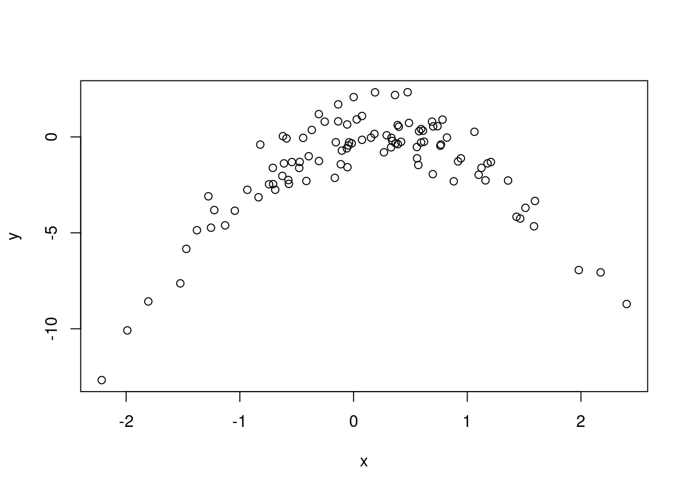

The plot is quadratic. X from about -2 to 2. Y from about -10 to 2.

We find the LOOCV MSEs using cv.glm from package boot. This requires to fit our models with glm() rather than lm(). But a linear model is a special case of GLM, so that’s not an issue.

library("boot")
myData <- data.frame(Y = y, X1 = x, X2 = x^2, X3 = x^3, X4 = x^4)
#initialise vector of LOOCV MSE (to compute for each of the 4 models)
errors <- c() 
set.seed(1)
fit <- glm(Y ~ X1, data = myData)
errors[1] <- cv.glm(myData[,1:2], fit)$delta[1] #keep only Y,X1 in myData

fit <- glm(Y ~ X1 + X2, data = myData)
errors[2] <- cv.glm(myData[,1:3], fit)$delta[1]

fit <- glm(Y ~ X1 + X2 + X3, data = myData)
errors[3] <- cv.glm(myData[,1:4], fit)$delta[1]

fit <- glm(Y ~ X1 + X2 + X3 + X4, data = myData)
errors[4] <- cv.glm(myData, fit)$delta[1]

print(round(errors,4))

[1] 7.2882 0.9374 0.9566 0.9539

Note that we could have used the “shortcut formula” instead, since we are in the case of linear regression. Let’s do it, using lm() to fit our models (just to convince you it’s equivalent). We obtain the same results… maths work!

#initialise vector of LOOCV MSE (to compute for each of the 4 models)
errors <- c()
fit <- lm(Y ~ X1, data = myData)
fit.hat <- hat(myData$X1)
# LOOCV shortcut for linear models
errors[1] <- mean(((myData$Y - fit$fitted.values) / (1 - fit.hat))^2)
# summary(fit)

fit <- lm(Y ~ X1 + X2, data = myData)
fit.hat <- hat(cbind(myData$X1, myData$X2))
errors[2] <- mean(((myData$Y - fit$fitted.values) / (1 - fit.hat))^2)
# summary(fit)

fit <- lm(Y ~ X1 + X2 + X3, data = myData)
fit.hat <- hat(cbind(myData$X1, myData$X2, myData$X3))
errors[3] <- mean(((myData$Y - fit$fitted.values) / (1 - fit.hat))^2)
# summary(fit)

fit <- lm(Y ~ X1 + X2 + X3 + X4, data = myData)
fit.hat <- hat(cbind(myData$X1, myData$X2, myData$X3, myData$X4))
errors[4] <- mean(((myData$Y - fit$fitted.values) / (1 - fit.hat))^2)
# summary(fit)
print(round(errors,4))

[1] 7.2882 0.9374 0.9566 0.9539

Regardless of the seed chosen, LOOCV with cv.glm returned the same results. This makes sense because this method, unlike the “validation set” approach, does not imply any randomisation (since all possible “folds” of size 1 are used).
The second model with X^1 and X^2 as predictors. This is what was expected, since that is the model used to generate the data in the first place.
Use summary(fit) with the previous commands to quickly check coefficient estimate significance. The conclusions drawn by checking the parameter estimates’ significance is the same as that of LOOCV. For the “underfitted” model 1, the parameter is barely significant. For the “overfitted” models 3 and 4, the extra parameters (X^3, X^4) are not significant, suggesting that Y = X + X^2 is the best model to use.

Question

library(ISLR2)
# sample size (here we find it as the length of the first column)
n <- length(College[, 1])
set.seed(1)
train.index <- sample(n, 2/3*n)
train <- (seq(1, n) %in% train.index)

fit <- lm(Grad.Rate ~ ., data = College, subset = train)
pred <- predict(fit, newdata = College[!train, ])
mean((pred - College[!train, ]$Grad.Rate)^2) # test error

[1] 167.3604

mean(fit$residuals^2) # training error

[1] 156.4825

library(glmnet)

Loading required package: Matrix

Loaded glmnet 4.1-8

# Design Matrix (removing first column, i.e., the intercept)
X.design <- model.matrix(Grad.Rate ~ ., College)[, -1]
# Vector of responses
Y <- as.matrix(College$Grad.Rate)  
# Ridge fit
fit.rdg <- glmnet(X.design[train, ], Y[train], alpha = 0)
plot(fit.rdg, xvar="lambda", label=T)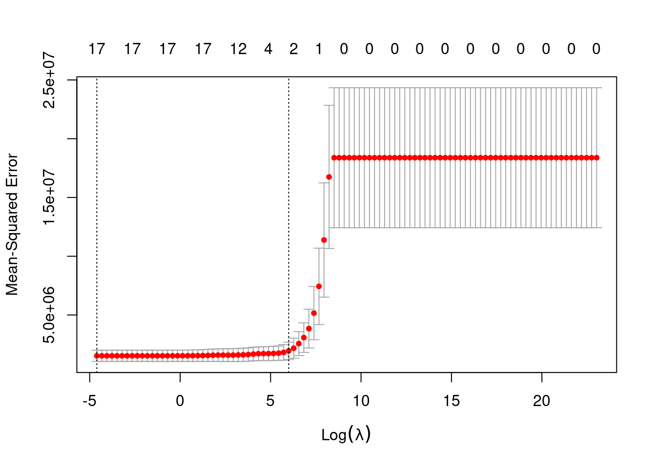

# Predictions on test set, with lambda=10
pred.rdg.10 <- predict(fit.rdg, s=10, newx = X.design[!train,])
mean((pred.rdg.10 - Y[!train])^2)

[1] 168.9593

# Ridge fit with cross-validated "lambda"
set.seed(1)
cv.rdg <- cv.glmnet(X.design[train, ], Y[train], alpha = 0)
plot(cv.rdg)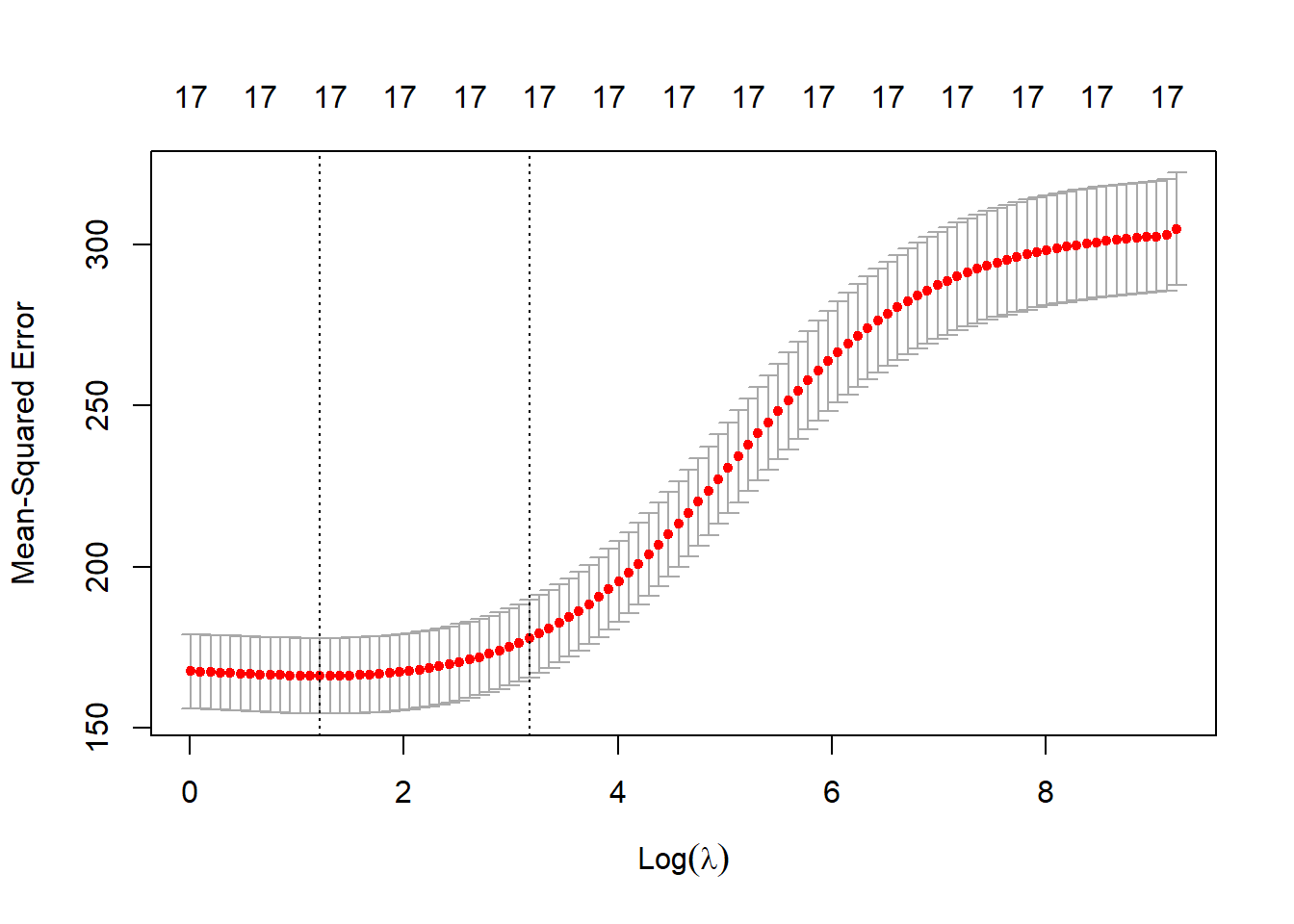

# Display optimal "lambda"
cv.rdg$lambda.min

[1] 3.384213

# Compute test MSE, under the optimised lambda
pred.rdg <- predict(cv.rdg, newx=X.design[!train,], s= cv.rdg$lambda.min)
(rdg.mse <- mean((pred.rdg - Y[!train])^2))

[1] 167.3224

The test mean-squared error is 167.32, essentially the same as under the initial linear regression model.

We do exactly the same thing, only now with \alpha=1 (which corresponds to Lasso regularisation).

# Lasso fit
fit.lso <- glmnet(X.design[train, ], Y[train], alpha = 1)
plot(fit.lso, xvar="lambda", label=T)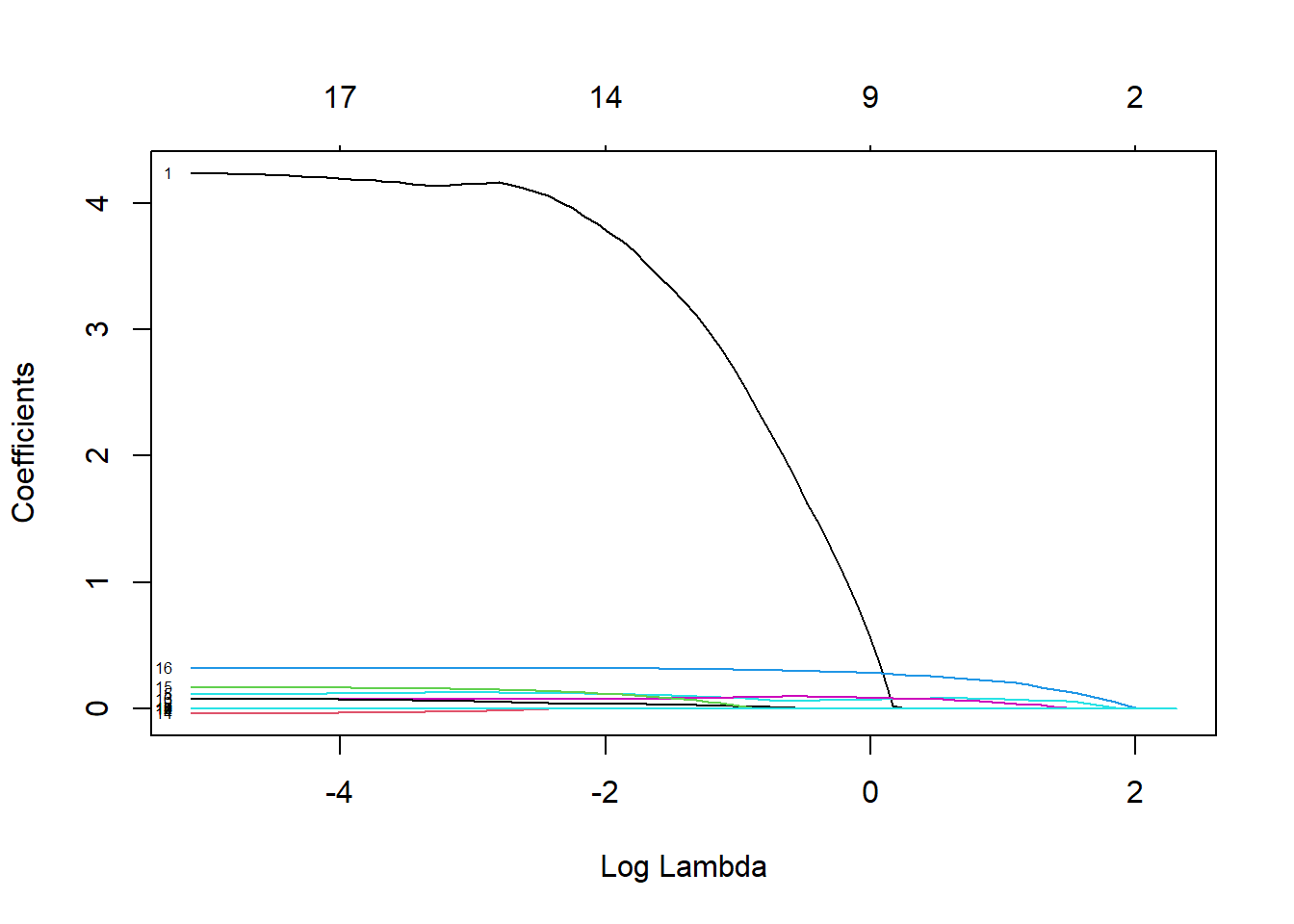

# Lasso fit with cross-validated "lambda"
set.seed(1)
cv.lso <- cv.glmnet(X.design[train, ], Y[train], alpha = 1)
plot(cv.lso)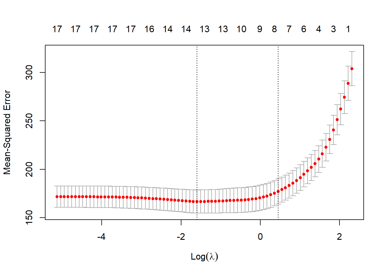

# Display optimal "lambda"
cv.lso$lambda.min

[1] 0.2028782

# Compute test MSE, under the optimised lambda
pred.lso <- predict(cv.lso, newx=X.design[!train,], s= cv.lso$lambda.min)
(lso.mse <- mean((pred.lso - Y[!train])^2))

[1] 166.7529

# Display lasso coefficients
coef(cv.lso, s = "lambda.min")

18 x 1 sparse Matrix of class "dgCMatrix"
                       s1
(Intercept)  3.406599e+01
PrivateYes   3.421914e+00
Apps         7.287893e-04
Accept       .           
Enroll       3.070244e-06
Top10perc    1.062188e-01
Top25perc    7.933764e-02
F.Undergrad  .           
P.Undergrad -1.478758e-03
Outstate     7.057560e-04
Room.Board   2.084713e-03
Books       -1.998945e-03
Personal    -2.547397e-03
PhD          3.263876e-02
Terminal     .           
S.F.Ratio    9.189933e-02
perc.alumni  3.155850e-01
Expend      -2.318226e-04

The test MSE has dropped a little bit, to 166.75. We note that three \beta coefficients have been pushed to 0.

The test MSE in the case of Lasso is the lowest, hence the best. However, all three models have achieved close MSE values, and so this is not an example where regularisation is “really” needed. About how well the model is performing: note that the MSE is a squared measure, so for better interpretation we should take its square root. Taking the square root of the lasso MSE, we get the value 12.91. This means that our prediction is typically “off” by that amount of percentage points (because the response is measured in percentage points). Also, note the R^2 of the linear model was 0.468 (and the linear model is close to the “best model”). So overall, we may declare as in that TV show: “not great, not terrible”.

Question

# Number of observations/predictors
n <- 1000
p <- 20
set.seed(1)
# Randomly generate the number of predictors that are significant ("non zero")
n.beta <- rbinom(1, p, 0.5)
# Create vector of 20 "betas" plus an intercept of "5" (arbitrary choice)
# Note all the "0" betas are a the end of the vector (arbitrary choice)
beta.vec <- c(5, runif(n.beta, min=-2, max=2), rep(0,p-n.beta))
# Randomly create entries of the design matrix to be number between 0 and 1
# (arbitrary choice)
myData  <- cbind(rep(1,n), matrix(runif(n * p), nrow = n, ncol = p))
# Create the response with Student noises for a change
Y <- myData %*% beta.vec + rt(n, df=30)
myData <- data.frame(Y = Y, myData[,-1])
linear.fit <- lm(Y ~ ., data=myData)
summary(linear.fit)


Call:
lm(formula = Y ~ ., data = myData)

Residuals:
    Min      1Q  Median      3Q     Max 
-3.2866 -0.7113 -0.0195  0.7563  3.2104 

Coefficients:
             Estimate Std. Error t value Pr(>|t|)    
(Intercept)  4.799706   0.266810  17.989  < 2e-16 ***
X1          -0.306590   0.120399  -2.546 0.011034 *  
X2           0.302795   0.117001   2.588 0.009797 ** 
X3           1.782867   0.119344  14.939  < 2e-16 ***
X4          -1.196736   0.115076 -10.400  < 2e-16 ***
X5           1.788535   0.118649  15.074  < 2e-16 ***
X6           1.771781   0.123110  14.392  < 2e-16 ***
X7           0.790965   0.120968   6.539 9.98e-11 ***
X8           0.466229   0.120246   3.877 0.000113 ***
X9          -1.737370   0.120944 -14.365  < 2e-16 ***
X10         -0.043213   0.117668  -0.367 0.713517    
X11         -0.039042   0.122065  -0.320 0.749151    
X12          0.003608   0.120265   0.030 0.976071    
X13          0.137173   0.118458   1.158 0.247151    
X14         -0.232691   0.120344  -1.934 0.053458 .  
X15          0.136257   0.122819   1.109 0.267526    
X16         -0.098169   0.118605  -0.828 0.408042    
X17          0.011574   0.121708   0.095 0.924256    
X18          0.011932   0.120516   0.099 0.921149    
X19         -0.157834   0.120038  -1.315 0.188863    
X20         -0.006997   0.119426  -0.059 0.953290    
---
Signif. codes:  0 '***' 0.001 '**' 0.01 '*' 0.05 '.' 0.1 ' ' 1

Residual standard error: 1.087 on 979 degrees of freedom
Multiple R-squared:  0.5183,    Adjusted R-squared:  0.5085 
F-statistic: 52.67 on 20 and 979 DF,  p-value: < 2.2e-16

set.seed(1)
train.index <- sample(1000, 100)
train <- (seq(1, 1000) %in% train.index)

library(leaps)
fit3 <- regsubsets(x = myData[, -1], y = Y, nvmax = p)
fit3.sum <- summary(fit3)
trainMSE <- rep(0, 20)
for (i in 1:20) {
  currfit     <- lm(Y ~ ., data = myData[train, fit3.sum$which[i, ]])
  trainMSE[i] <- mean((Y[train] - currfit$fitted.values)^2)
}
plot(seq(1:20), trainMSE, type = "l", col="brown3", lwd=2, xlab="number of predictors")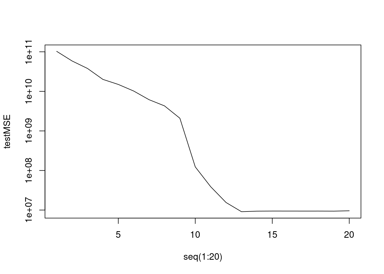

testMSE <- rep(0, 20)
for (i in 1:20) {
  currfit <- lm(Y ~ ., data = myData[train, fit3.sum$which[i, ]])
  testMSE[i] <- mean((Y[!train] - predict(currfit, newdata = myData[!train, ]))^2)
}
plot(seq(1:20), testMSE, type = "l", col="brown3", lwd=2, xlab="number of predictors")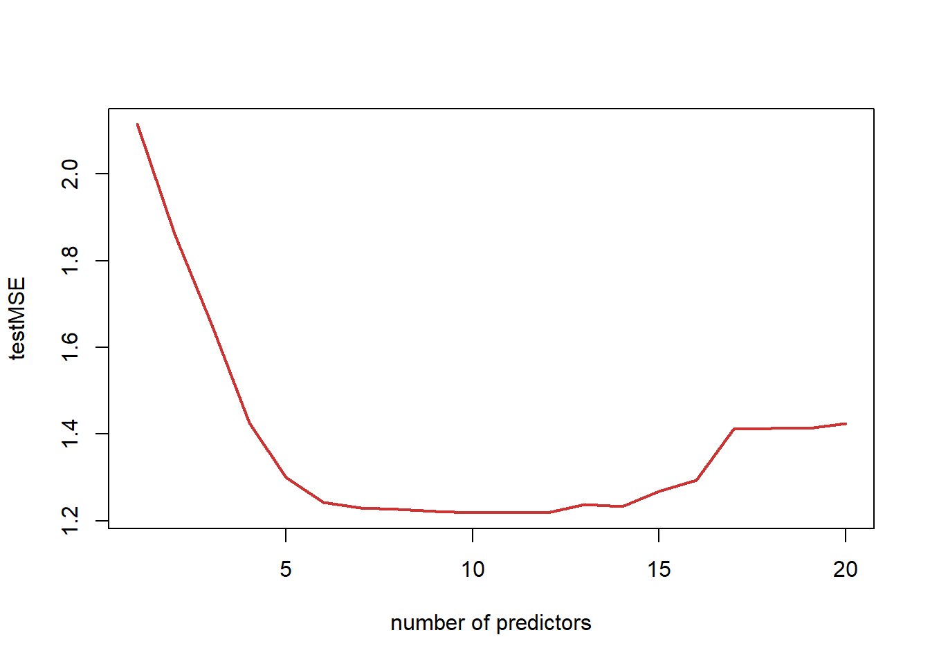

print(testMSE)

 [1] 2.114720 1.861551 1.650669 1.426621 1.299746 1.242543 1.228922 1.226431
 [9] 1.222030 1.218108 1.219055 1.218249 1.237309 1.232803 1.268381 1.293093
[17] 1.411646 1.412922 1.413230 1.424872

min(testMSE)

[1] 1.218108

```
coef(fit3, 10)
```
```
(Intercept)          X1          X2          X3          X4          X5 
  4.7818419  -0.3064279   0.2905511   1.7783451  -1.1974747   1.7936418 
         X6          X7          X8          X9         X14 
  1.7699818   0.8035569   0.4571409  -1.7478968  -0.2273410 
```
In this case, the test MSE is minimised for the model with 10 predictors. As expected, the training MSE keeps decreasing as we add predictors. The test MSE decreases at first, but then starts increasing when we are adding too many predictors that are not truly related to the response (i.e., we are overfitting).
The model’s estimates are relatively close to the true coefficients in the vector beta.vec. We note that the last predictor in this best model (X14) is not “supposed” to be significant.

# Design Matrix (removing the intercept)
X.design <- model.matrix(Y ~ ., myData)[, -1]
set.seed(1)
cv.lso <- cv.glmnet(X.design, Y, alpha = 1)
plot(cv.lso)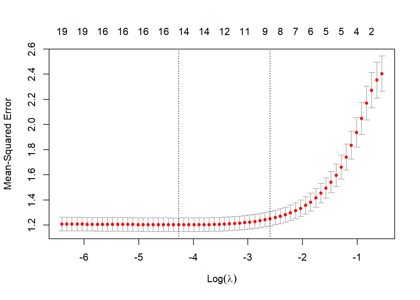

coef(cv.lso, s="lambda.min")

21 x 1 sparse Matrix of class "dgCMatrix"
                     s1
(Intercept)  4.82534161
X1          -0.25559214
X2           0.25365223
X3           1.73149691
X4          -1.14785385
X5           1.74692543
X6           1.71947501
X7           0.74050723
X8           0.41101469
X9          -1.68496783
X10          .         
X11          .         
X12          .         
X13          0.09372722
X14         -0.17761310
X15          0.07424414
X16         -0.05503574
X17          .         
X18          .         
X19         -0.11687289
X20          .

The Lasso has correctly identified variables X1 to X9 as significant. However, it has also left in the model several variables that should not be there, which is a little underwhelming.