Moving Beyond Linearity

library(tidyverse)
library(splines)
library(mgcv)

import pandas as pd
import numpy as np
import matplotlib.pyplot as plt
import seaborn as sns

from patsy import dmatrix
import statsmodels.api as sm
import statsmodels.formula.api as smf

Disclaimer

Some of the figures in this presentation are taken from “An Introduction to Statistical Learning, with applications in R” (Springer, 2021) with permission from the authors: G. James, D. Witten, T. Hastie and R. Tibshirani.

Overview

• Linearity & Nonlinearity
• Data Science Starts With Data
• Linear Regression
• Polynomial Regression
• Step Functions
• Regression Splines
• Smoothing Splines
• Local Regression
• Generalised Additive Models (GAMs)

Reading

James et al. (2021): Chapter 7

Linearity & Nonlinearity

Nonlinear curves

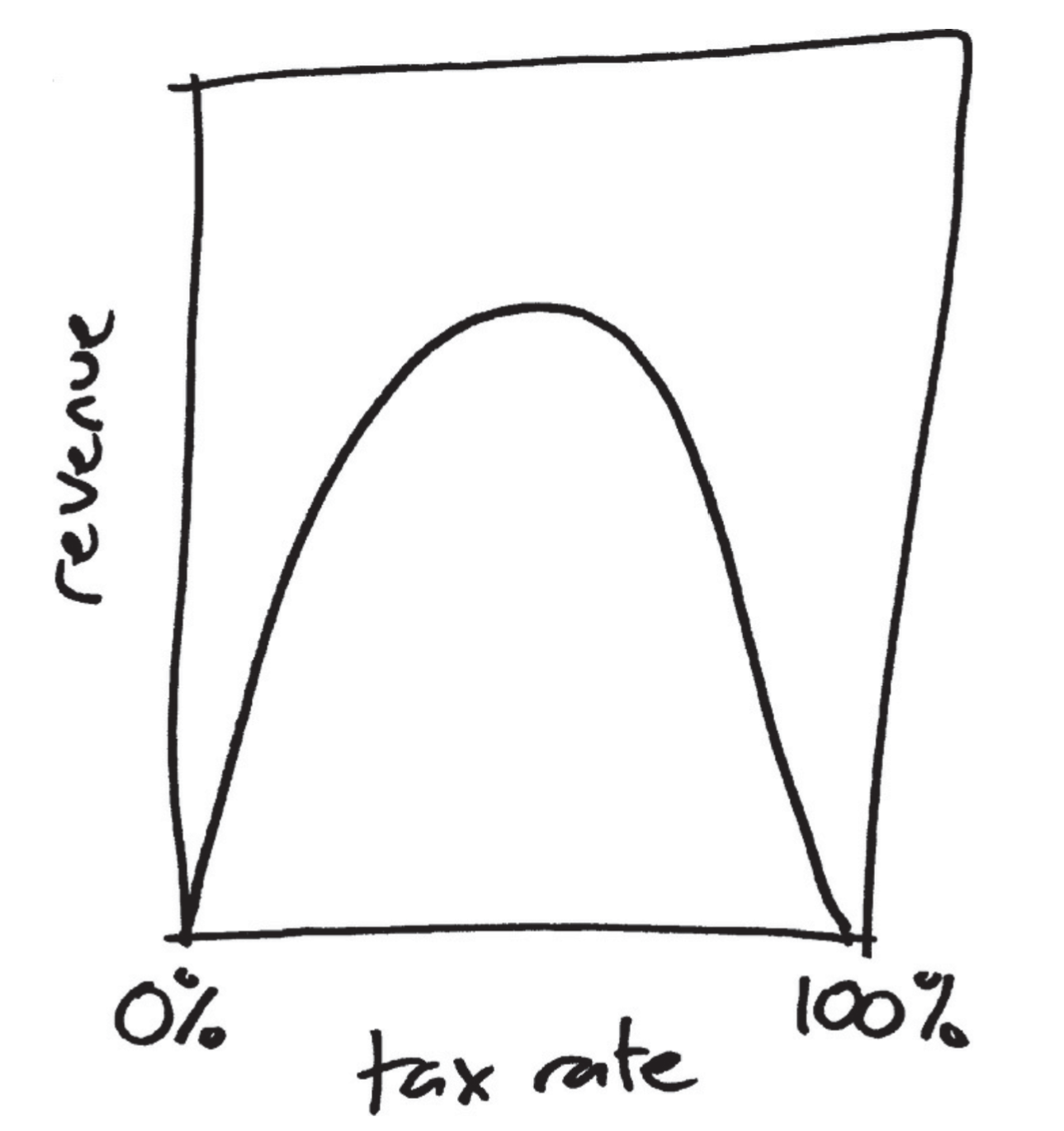
The legend of the Laffer curve goes like this: Arthur Laffer, then an economics professor at the University of Chicago, had dinner one night in 1974 with Dick Cheney, Donald Rumsfeld, and Wall Street Journal editor Jude Wanniski at an upscale hotel restaurant in Washington DC. They were tussling over President Ford’s tax plan, and eventually, as intellectuals do when the tussling gets heavy, Laffer commandeered a napkin and drew a picture. The picture looked like this:

Laffer curve

Source: Jordan Ellenberg (2014), How Not to Be Wrong: The Power of Mathematical Thinking

One predictor vs multiple predictors

\texttt{sales} \approx \beta_0 + \beta_1 \times \texttt{TV}

Linear regression

\texttt{sales} \approx \beta_0 + \beta_1 \times \texttt{TV}+ \beta_2 \times \texttt{radio}

Multiple linear regression

Source: James et al. (2021), An Introduction to Statistical Learning with Applications in R, Figures 3.1 & 3.5.

By the end of today

Instead of just fitting lines (linear regression) or hyperplanes (multiple linear regression)…

You’ll be able to fit nonlinear curves to multivariate data using splines and Generalised Additive Models.

We’ll focus on one predictor and one response variable for most of this lecture.

Source: James et al. (2021), An Introduction to Statistical Learning with Applications in R, Figures 2.4 & 2.6.

Moving beyond linearity

Using a term like nonlinear science is like referring to the bulk of zoology as the study of non-elephant animals. (Stanisław Ulam)

• Linear models are highly interpretable, but can be very unrealistic.
• Ideally, we would want interpretable nonlinear models. But, from a machine learning view (not a statistical view), we care more about predictions.
• Here we cover:
  1. Polynomial regression
  2. Step functions
  3. Regression splines
  4. Smoothing splines
  5. Local regression
  6. Generalised additive models

Data Science Starts With Data

Luxembourg Mortality Data

Download a file called Mx_1x1.txt from the Human Mortality Database.

No-one is allowed to distribute the data, but you can download it for free. Here are the first few rows to get a sense of what it looks like.

with open('Mx_1x1.txt', 'r') as file:
    for i in range(10):
        print(file.readline(), end='')

Luxembourg, Death rates (period 1x1),   Last modified: 09 Aug 2023;  Methods Protocol: v6 (2017)

  Year          Age             Female            Male           Total
  1960           0             0.023863        0.039607        0.031891
  1960           1             0.001690        0.003528        0.002644
  1960           2             0.001706        0.002354        0.002044
  1960           3             0.001257        0.002029        0.001649
  1960           4             0.000844        0.001255        0.001051
  1960           5             0.000873        0.001701        0.001293
  1960           6             0.000443        0.000430        0.000437

Setup & importing the data

R

lux <- read_table("Mx_1x1.txt", skip = 2, show_col_types = FALSE) %>%
  rename(age=Age, year=Year, mx=Female) %>%
  select(age, year, mx) %>%
  filter(age != '110+') %>%
  mutate(year = as.integer(year), age = as.integer(age), mx = as.numeric(mx))

lux

# A tibble: 6,930 × 3
     age  year       mx
   <int> <int>    <dbl>
 1     0  1960 0.0239  
 2     1  1960 0.00169 
 3     2  1960 0.00171 
 4     3  1960 0.00126 
 5     4  1960 0.000844
 6     5  1960 0.000873
 7     6  1960 0.000443
 8     7  1960 0       
 9     8  1960 0.000951
10     9  1960 0       
# ℹ 6,920 more rows

summary(lux)

      age             year            mx         
 Min.   :  0.0   Min.   :1960   Min.   :0.00000  
 1st Qu.: 27.0   1st Qu.:1975   1st Qu.:0.00045  
 Median : 54.5   Median :1991   Median :0.00337  
 Mean   : 54.5   Mean   :1991   Mean   :0.09200  
 3rd Qu.: 82.0   3rd Qu.:2007   3rd Qu.:0.04178  
 Max.   :109.0   Max.   :2022   Max.   :6.00000  
                                NA's   :358      

Python

lux = pd.read_csv('Mx_1x1.txt', sep='\s+', skiprows=2)

lux = lux.rename(columns={'Age': 'age', 'Year': 'year', 'Female': 'mx'})
lux = lux[['age', 'year', 'mx']]
lux = lux[lux['age'] != '110+'].copy()
lux.loc[lux['mx'] == '.', 'mx'] = np.nan

lux['year'] = lux['year'].astype(int)
lux['age'] = lux['age'].astype(int)
lux['mx'] = lux['mx'].astype(float)

lux

      age  year        mx
0       0  1960  0.023863
1       1  1960  0.001690
2       2  1960  0.001706
3       3  1960  0.001257
4       4  1960  0.000844
...   ...   ...       ...
6987  105  2022  0.661481
6988  106  2022  5.419704
6989  107  2022       NaN
6990  108  2022       NaN
6991  109  2022       NaN

[6930 rows x 3 columns]

Mortality

R

average_df <- lux %>% group_by(age) %>% summarise(mx = mean(mx, na.rm = TRUE))
ggplot(lux, aes(x = age, y = mx)) +
  geom_line(aes(group = year, color = year), alpha = 0.3) +
  geom_line(data = average_df, color = "black", linewidth = 1) +
  labs(x = "Age", y = "Mortality Rate", color = "Year") +
  theme_minimal()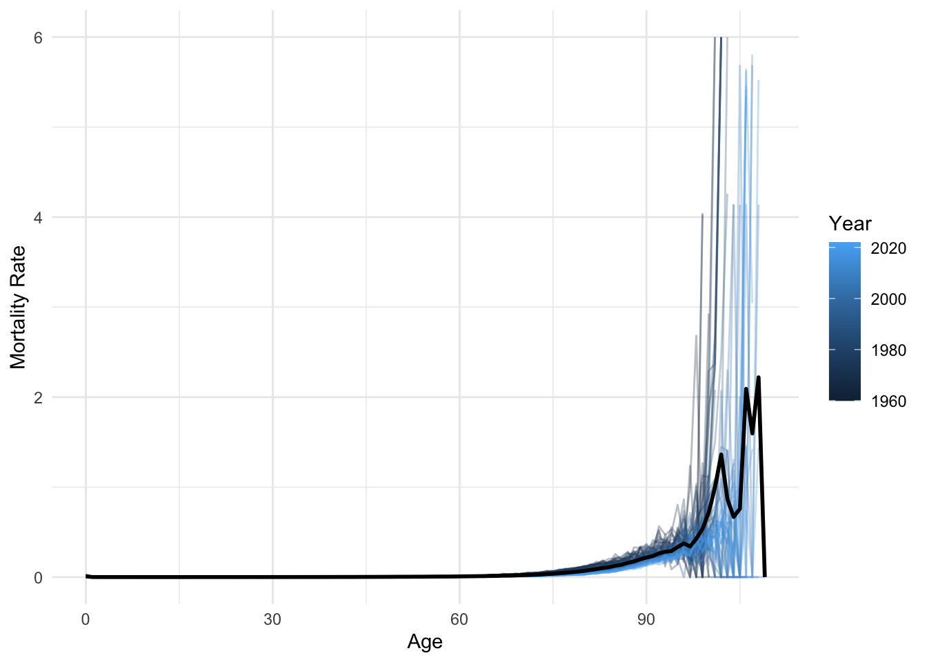

Python

average_df = lux.groupby('age')[['mx']].mean().reset_index()
sns.lineplot(data=lux, x='age', y='mx', hue='year', palette='viridis', alpha=0.3)
plt.plot(average_df['age'], average_df['mx'], color='black', linewidth=2)
plt.xlabel('Age'); plt.ylabel('Mortality Rate');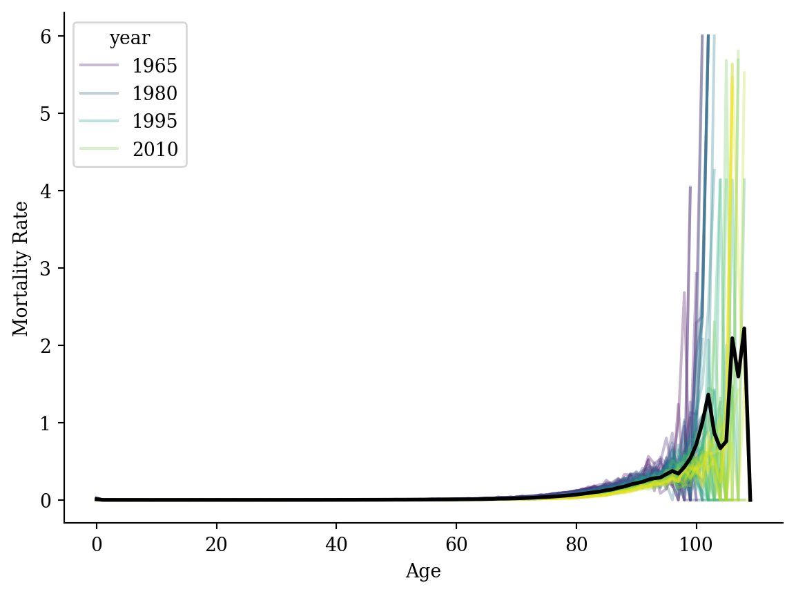

Mortality (zoom in)

R

lux <- lux %>% filter(age <= 90)

average_df <- average_df %>% filter(age <= 90)

ggplot(lux, aes(x = age, y = mx)) +
  geom_line(aes(group = year, color = year), alpha = 0.3) +
  geom_line(data = average_df, color = "black", linewidth = 1) +
  labs(x = "Age", y = "Mortality Rate", color = "Year") +
  theme_minimal()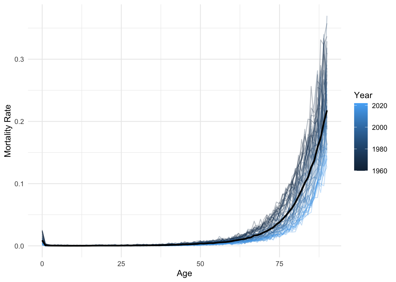

Python

lux = lux[lux['age'] <= 90].copy()

average_df = average_df[average_df['age'] <= 90]

sns.lineplot(data=lux, x='age', y='mx', hue='year', palette='viridis', alpha=0.3)
plt.plot(average_df['age'], average_df['mx'], color='black', linewidth=2)
plt.xlabel('Age'); plt.ylabel('Mortality Rate');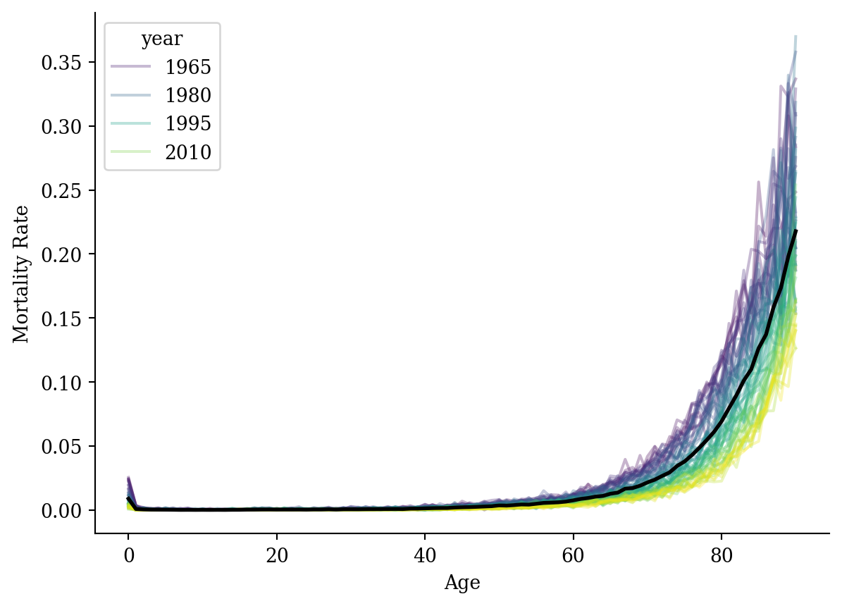

Log-mortality

R

lux$log_mx <- log(lux$mx)
lux <- lux[lux$log_mx != -Inf, ]

average_df <- average_df %>%
  left_join(lux %>%
              group_by(age) %>%
              summarise(log_mx = mean(log_mx, na.rm = TRUE)),
            by = "age")

ggplot(lux, aes(x = age, y = log_mx)) +
  geom_line(aes(group = year, color = year), alpha = 0.3) +
  geom_line(data = average_df, color = "black", linewidth = 1) +
  labs(x = "Age", y = "Log-Mortality Rate", color = "Year") +
  theme_minimal()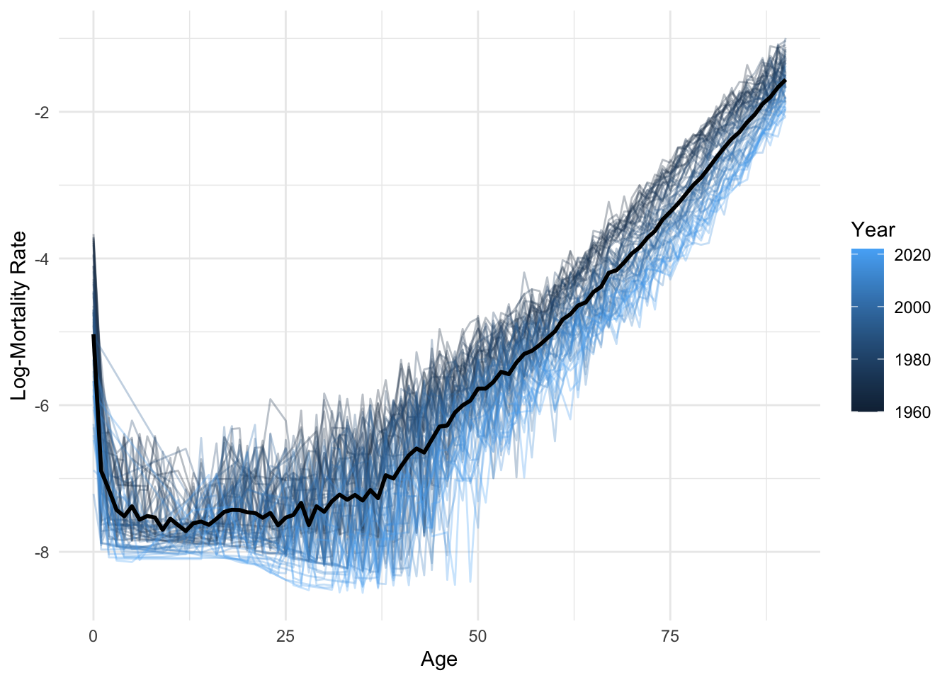

Python

lux['log_mx'] = np.log(lux['mx'])

C:\Users\Patrick\MAMBAF~1\envs\ml2025\Lib\site-packages\pandas\core\arraylike.py:399: RuntimeWarning: divide by zero encountered in log
  result = getattr(ufunc, method)(*inputs, **kwargs)

lux = lux[lux['log_mx'] != -np.inf]

average_df['log_mx'] = lux.groupby('age')[['log_mx']].mean()

sns.lineplot(data=lux, x='age', y='log_mx', hue='year', palette='viridis', alpha=0.3)
plt.plot(average_df['age'], average_df['log_mx'], color='black', linewidth=2)
plt.xlabel('Age'); plt.ylabel('Log-Mortality Rate');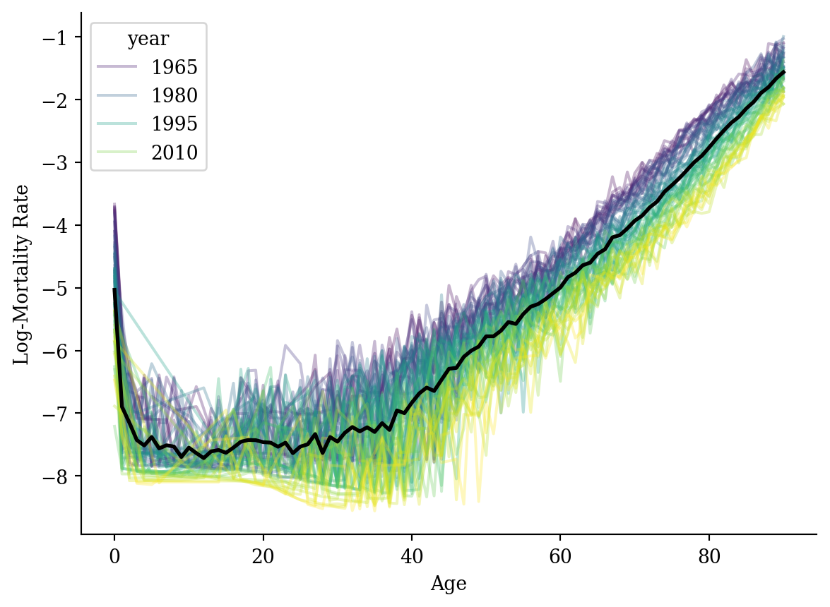

Linear regression

R

lux_2020 <- lux %>% filter(year == 2020)
model_lr <- lm(log_mx ~ age, data = lux_2020)

p <- ggplot(lux_2020, aes(x = age, y = log_mx)) + theme_minimal() +
  geom_point(alpha = 0.75) + labs(x = "Age", y = "Log-Mortality")

age_grid <- data.frame(age = seq(min(lux$age), max(lux$age), by=0.1))
predictions <- predict(model_lr, newdata = age_grid)

p + geom_line(data = age_grid, aes(x = age, y = predictions),
              color = "red", linewidth=2)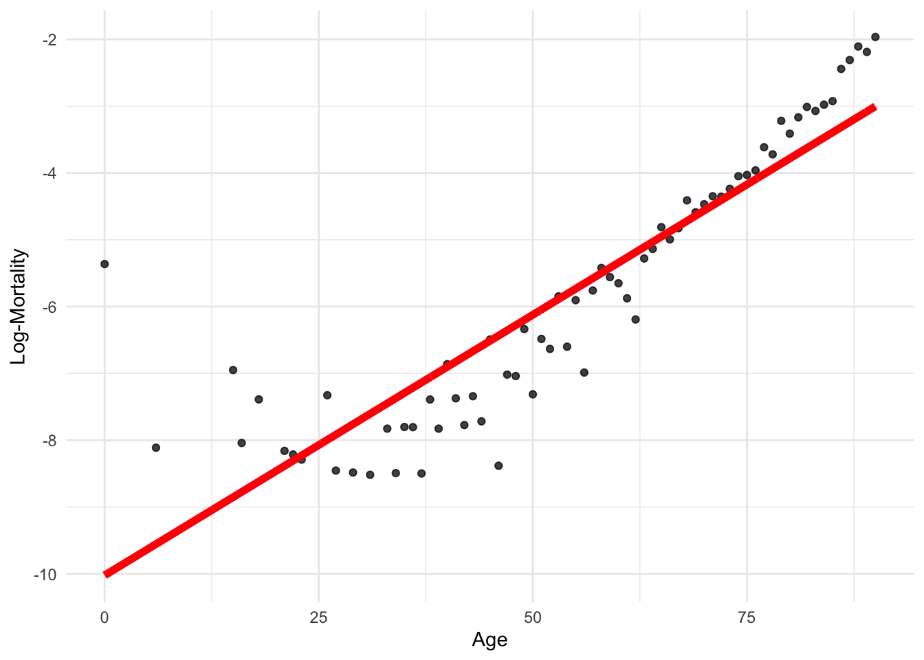

Python

lux_2020 = lux[lux['year'] == 2020].copy()
model_lr = smf.ols('log_mx ~ age', data=lux_2020).fit()

plt.scatter(lux_2020['age'], lux_2020['log_mx'], alpha=0.75)
plt.plot(lux_2020['age'], model_lr.predict(lux_2020[['age']]), color='red')
plt.xlabel('Age'); plt.ylabel('Log-Mortality');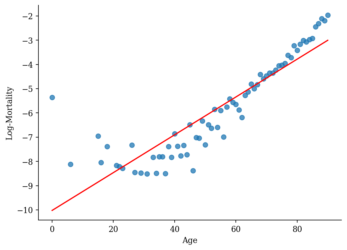

Quadratic regression

R

model_quad <- lm(log_mx ~ poly(age, 2), data = lux_2020)

predictions <- predict(model_quad, newdata = age_grid)
p + geom_line(data = age_grid, aes(x = age, y = predictions),
              color = "red", linewidth=2)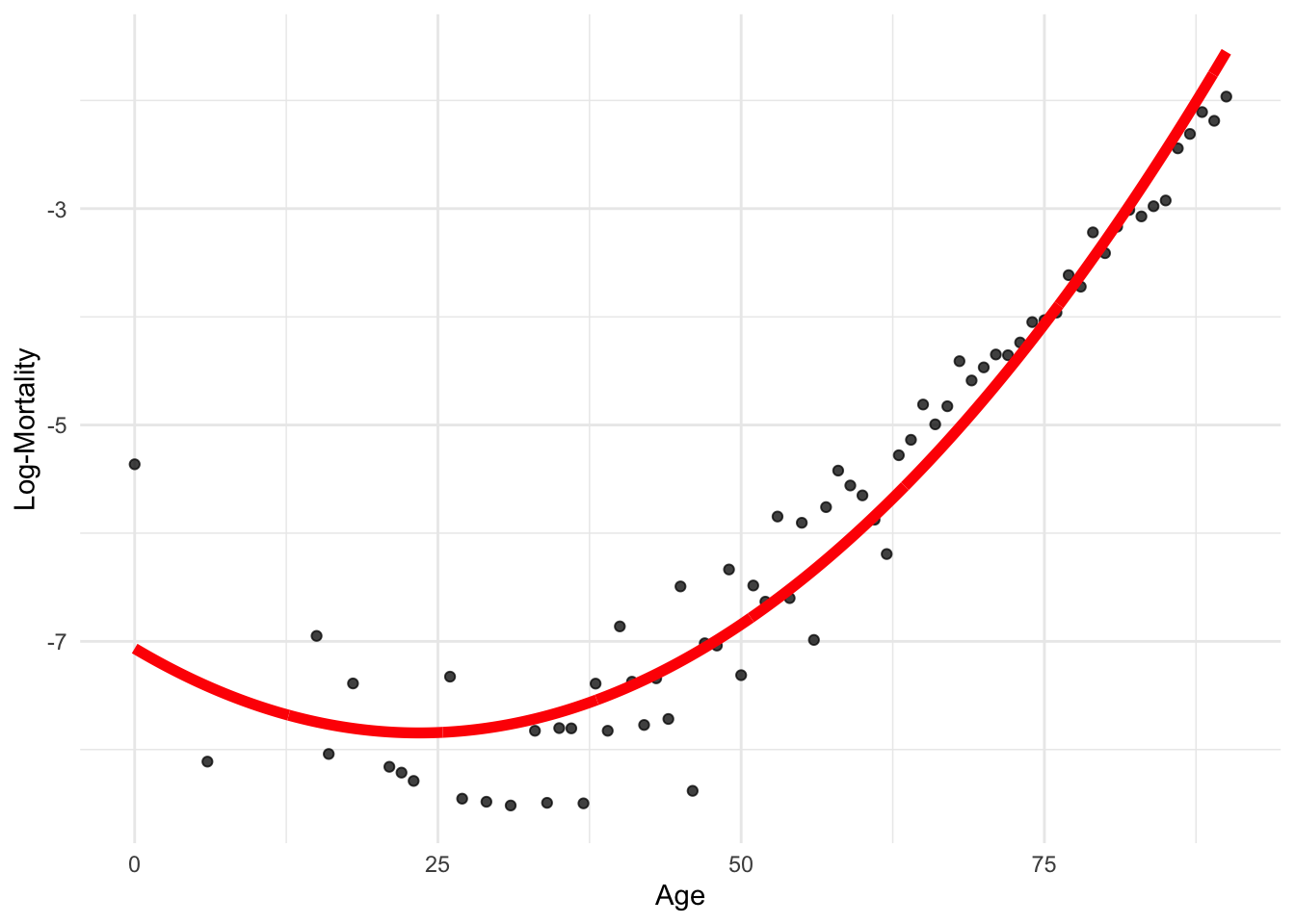

Python

model_quad = smf.ols('log_mx ~ np.power(age, 2) + age', data=lux_2020).fit()

plt.scatter(lux_2020['age'], lux_2020['log_mx'], alpha=0.75)
plt.plot(lux_2020['age'], model_quad.predict(lux_2020), color='red', linewidth=2)
plt.xlabel('Age'); plt.ylabel('Log Mortality');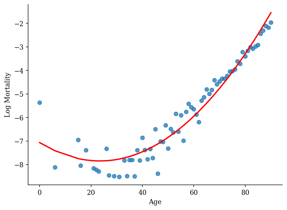

Step function regression

R

model_step <- lm(log_mx ~ cut(age, seq(0, 90, 10), right=F), data = lux_2020)

p <- ggplot(lux_2020, aes(x = age, y = log_mx)) + theme_minimal() +
  geom_point(alpha = 0.75) + labs(x = "Age", y = "Log-Mortality")

age_grid <- data.frame(age = seq(min(lux$age), max(lux$age), by=0.1))
predictions <- predict(model_step, newdata = age_grid)

p + geom_point(data = age_grid, aes(x = age, y = predictions),
              color = "red", size=2)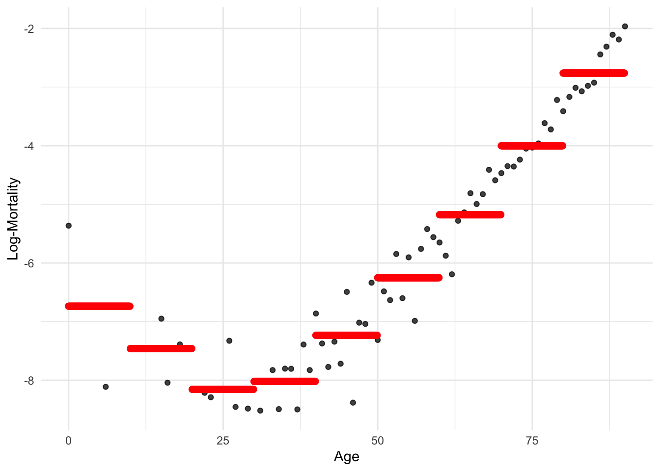

Python

lux_2020['age_bin'] = pd.cut(lux_2020['age'], bins=np.arange(0, 101, 10), right=False)
lux_2020['age_bin_str'] = lux_2020['age_bin'].astype(str)
model_step = smf.ols('log_mx ~ age_bin_str', data=lux_2020).fit()

# Generate a DataFrame for predictions
# This involves creating a DataFrame where 'age' spans the unique bins used in the model
age_grid = np.linspace(0, 101, 1000)

df_plot = pd.DataFrame({
  'age': age_grid,
  'age_bin_str': pd.cut(age_grid, bins=np.arange(0, 101, 10), right=False).astype(str)}
)

# Predict using the model
df_plot['predictions'] = model_step.predict(df_plot)

# Plot
plt.scatter(lux_2020['age'], lux_2020['log_mx'], alpha=0.75)
plt.scatter(df_plot['age'], df_plot['predictions'], color='red', linewidth=2)
plt.xlabel('Age')
plt.ylabel('Log-Mortality')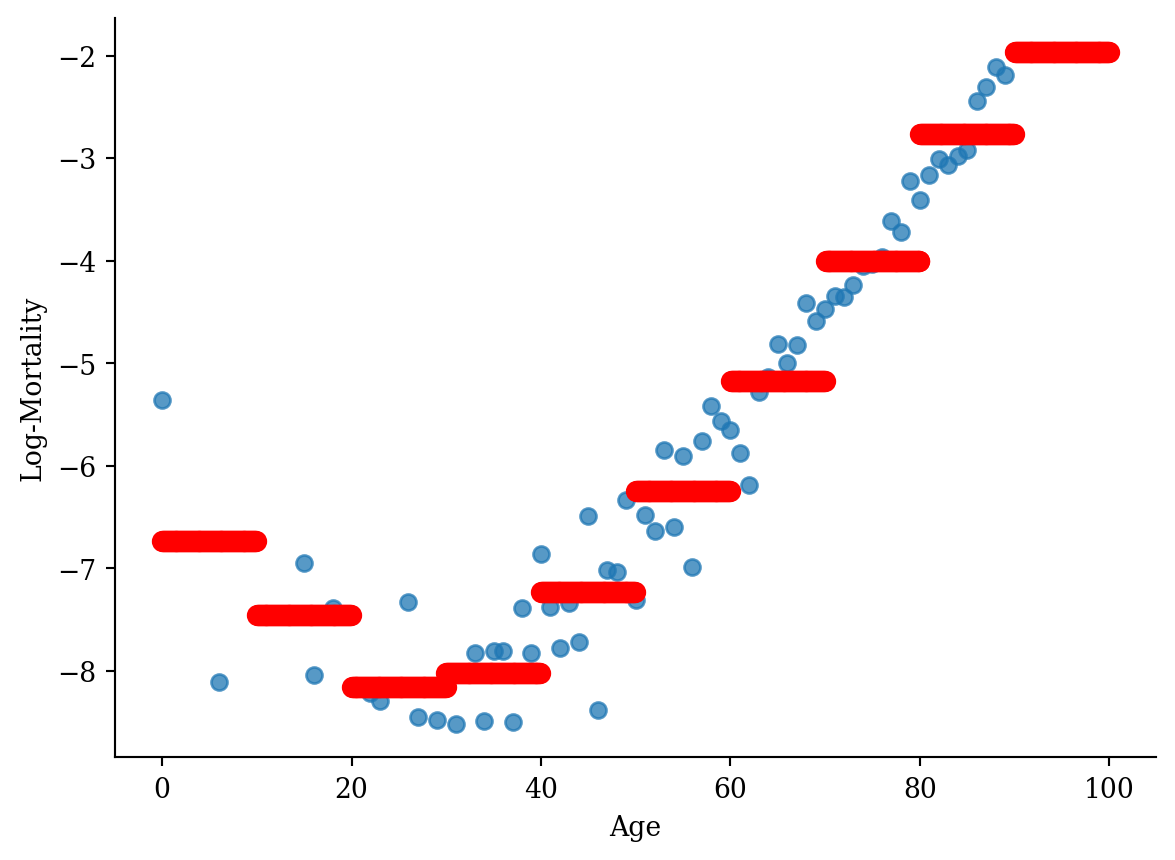

Regression spline

R

model_spline <- lm(log_mx ~ bs(age, degree=10), data=lux_2020) # Requires splines package

predictions <- predict(model_spline, newdata = age_grid)
p + geom_line(data = age_grid, aes(x = age, y = predictions),
              color = "red", linewidth=2, alpha=0.75)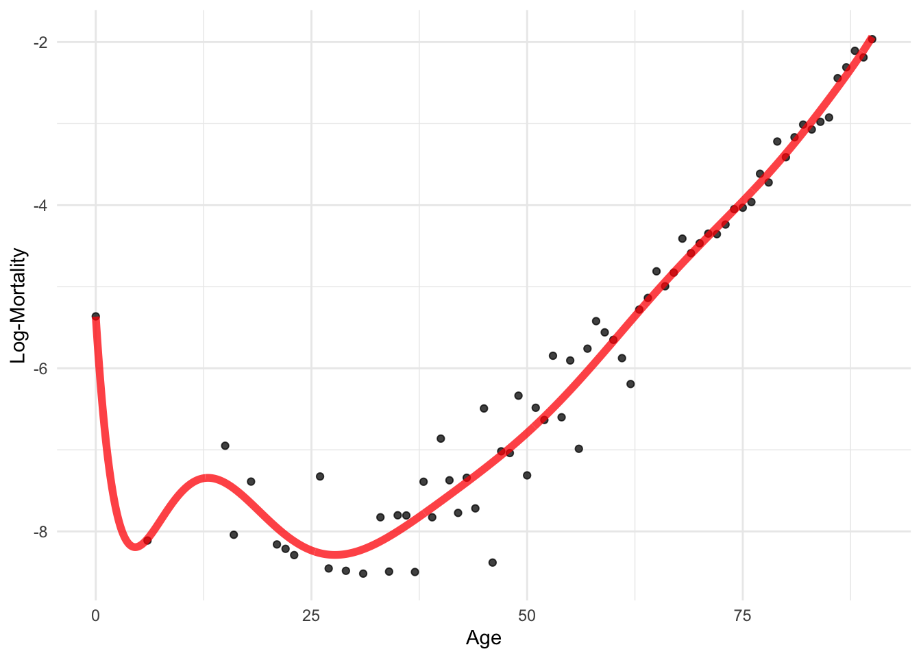

Python

spline_x = dmatrix("bs(lux_2020['age'], degree=3, knots=[15,30,45])",
    {"lux_2020['age']": lux_2020['age']}, return_type='dataframe')
model_spline = sm.GLM(lux_2020['log_mx'], spline_x).fit()

# Prepare data for plotting
x_range = pd.DataFrame({'age': np.linspace(lux_2020['age'].min(), lux_2020['age'].max(), 100)})
x_range_transformed = dmatrix("bs(x_range, degree=3, knots=[15,30,45])", {"x_range": x_range['age']}, return_type='dataframe')

predictions_spline = model_spline.predict(x_range_transformed)

plt.scatter(lux_2020['age'], lux_2020['log_mx'], alpha=0.75)
plt.plot(x_range['age'], predictions_spline, color='red')
plt.xlabel('Age'); plt.ylabel('Log Mortality');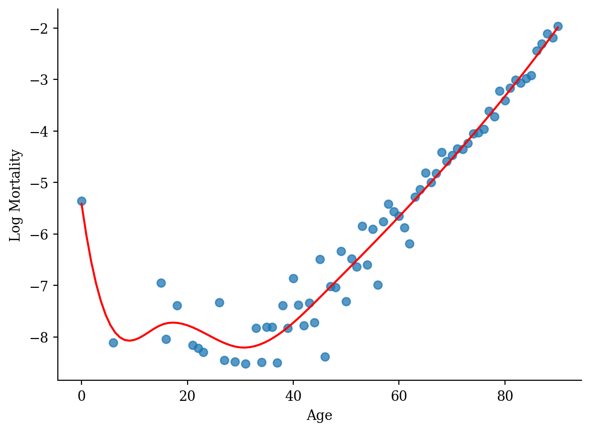

Industry approaches

IFoA bulletin on machine learning in mortality modelling

Methods from this class (p. 8–9):

• ridge regression
• lasso regression
• elastic net
• generalised linear models
• generalised additive models
• random forests
• dimension reduction
• (artificial neural networks)

Take ACTL3141/ACTL5104 for mortality modelling, ACTL3143/ACTL5111 for actuarial AI

Linear Regression

Plotting the fitted values

R

ggplot(lux_2020, aes(x = age, y = log_mx)) + theme_minimal() +
  geom_point(aes(y = predict(model_lr)), color = "red", size = 2) +
  geom_point(alpha = 0.75, size = 2) + labs(x = "Age", y = "Log-Mortality")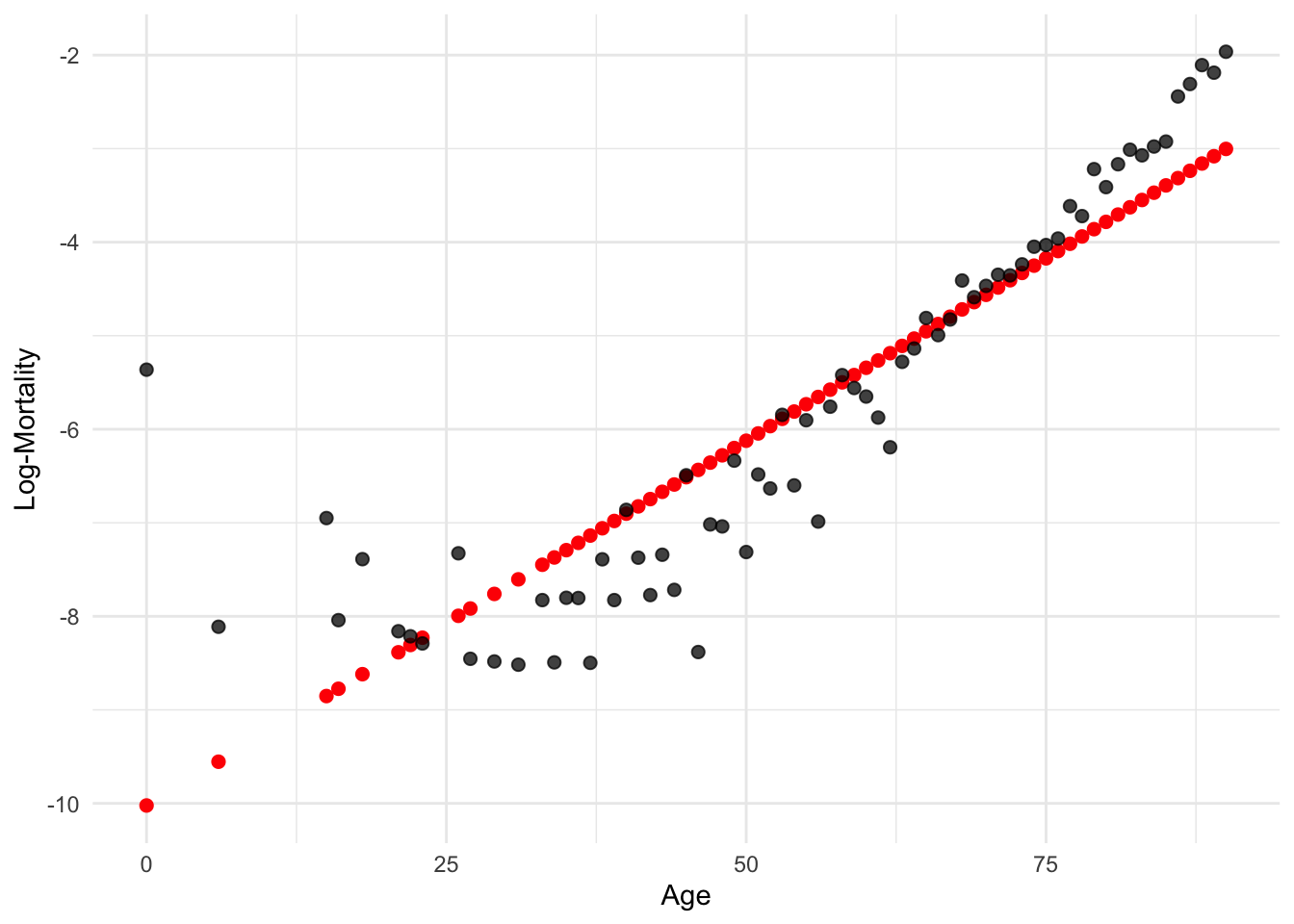

Python

model = smf.ols('log_mx ~ age', data=lux_2020).fit()
plt.scatter(lux_2020['age'], model.predict(lux_2020[['age']]), color='red')
plt.scatter(lux_2020['age'], lux_2020['log_mx'], alpha=0.75)
plt.xlabel('Age'); plt.ylabel('Log-Mortality');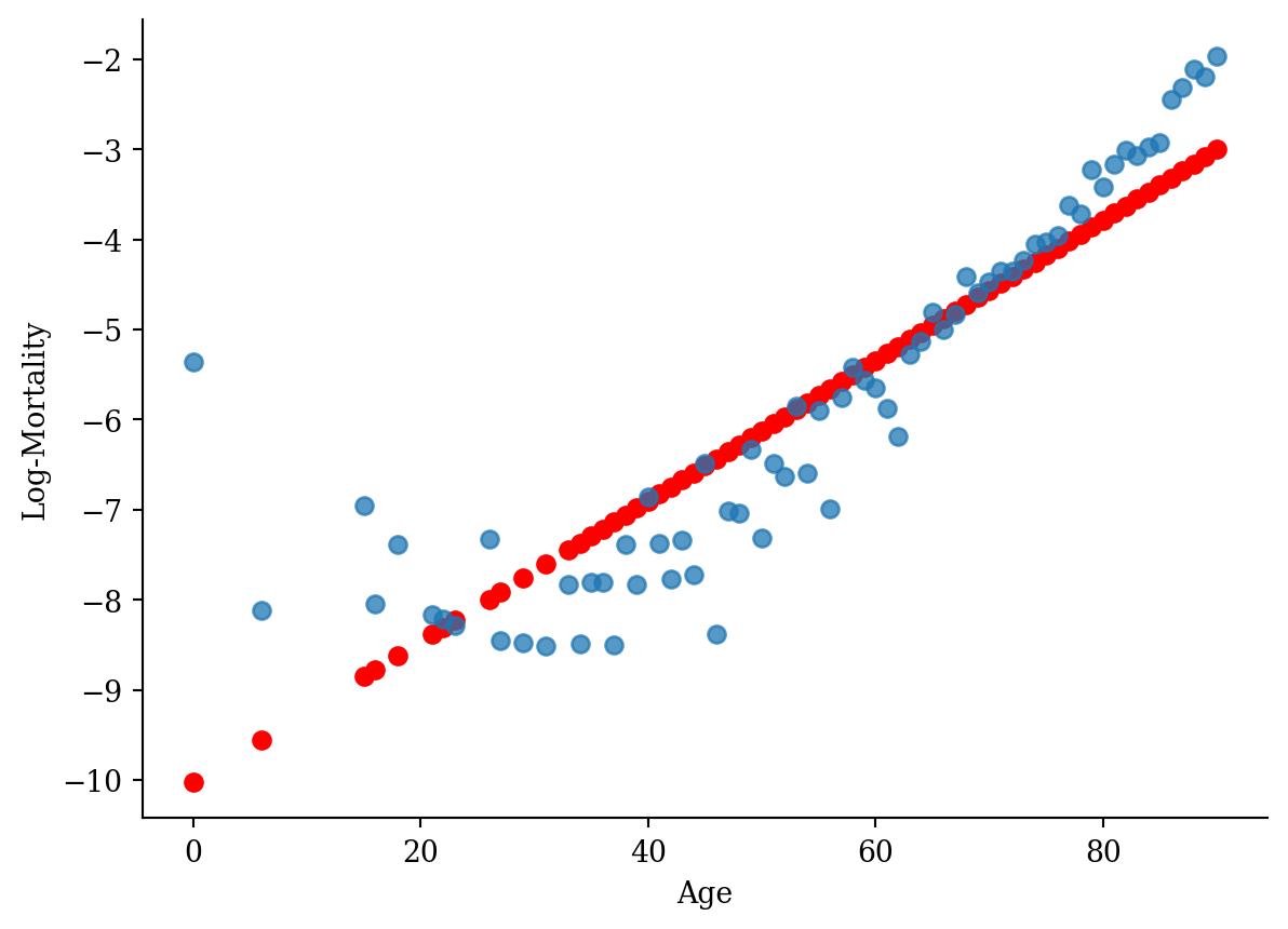

Linear regression with error bars

R

ggplot(lux_2020, aes(x = age, y = log_mx)) + theme_minimal() +
  geom_smooth(method = "lm", formula = y ~ x, color = "red", linewidth=2) +
  geom_point(alpha = 0.75) + labs(x = "Age", y = "Log Mortality")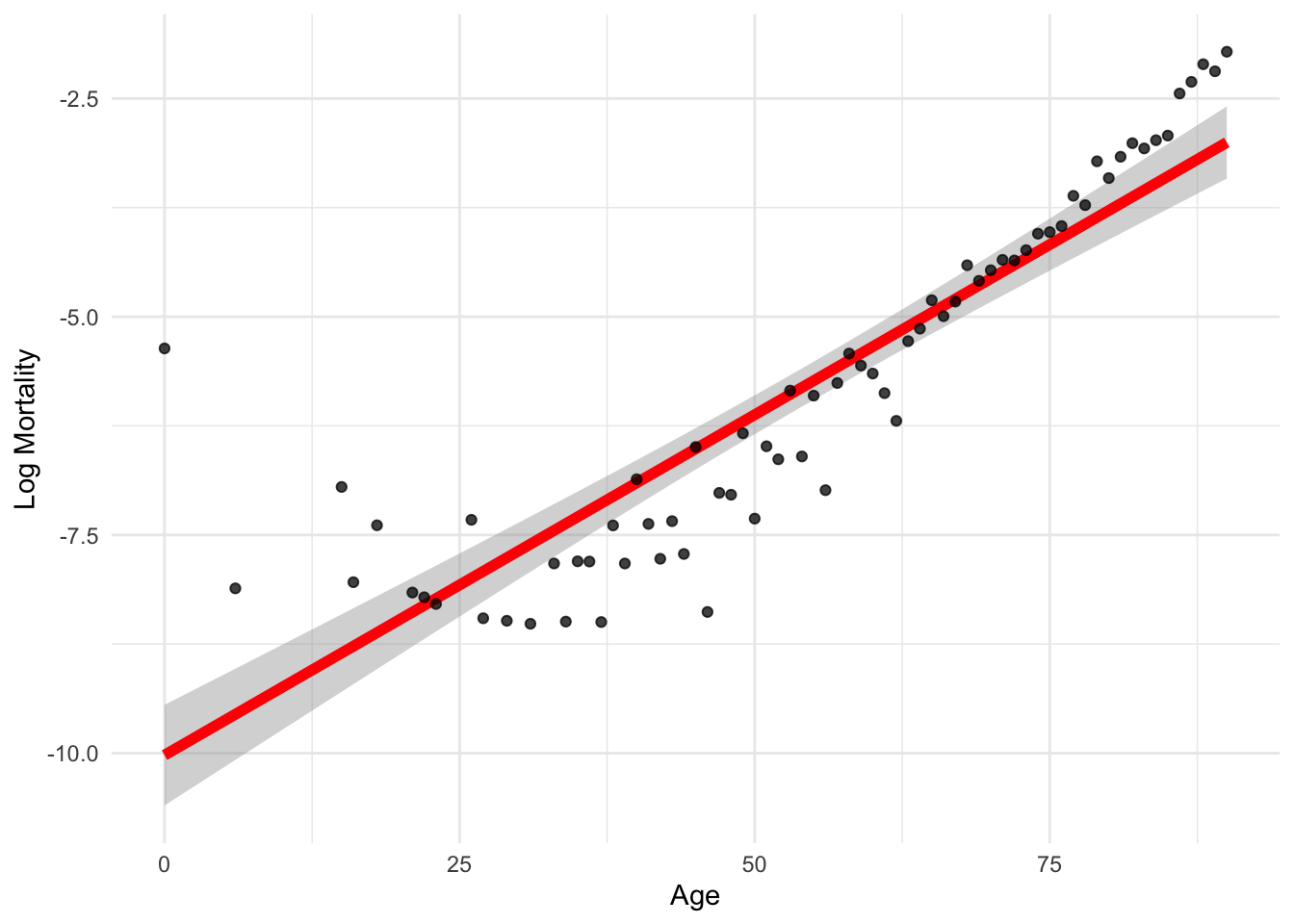

Python

sns.regplot(x='age', y='log_mx', data=lux_2020, ci=95)
plt.xlabel('Age'); plt.ylabel('Log-Mortality');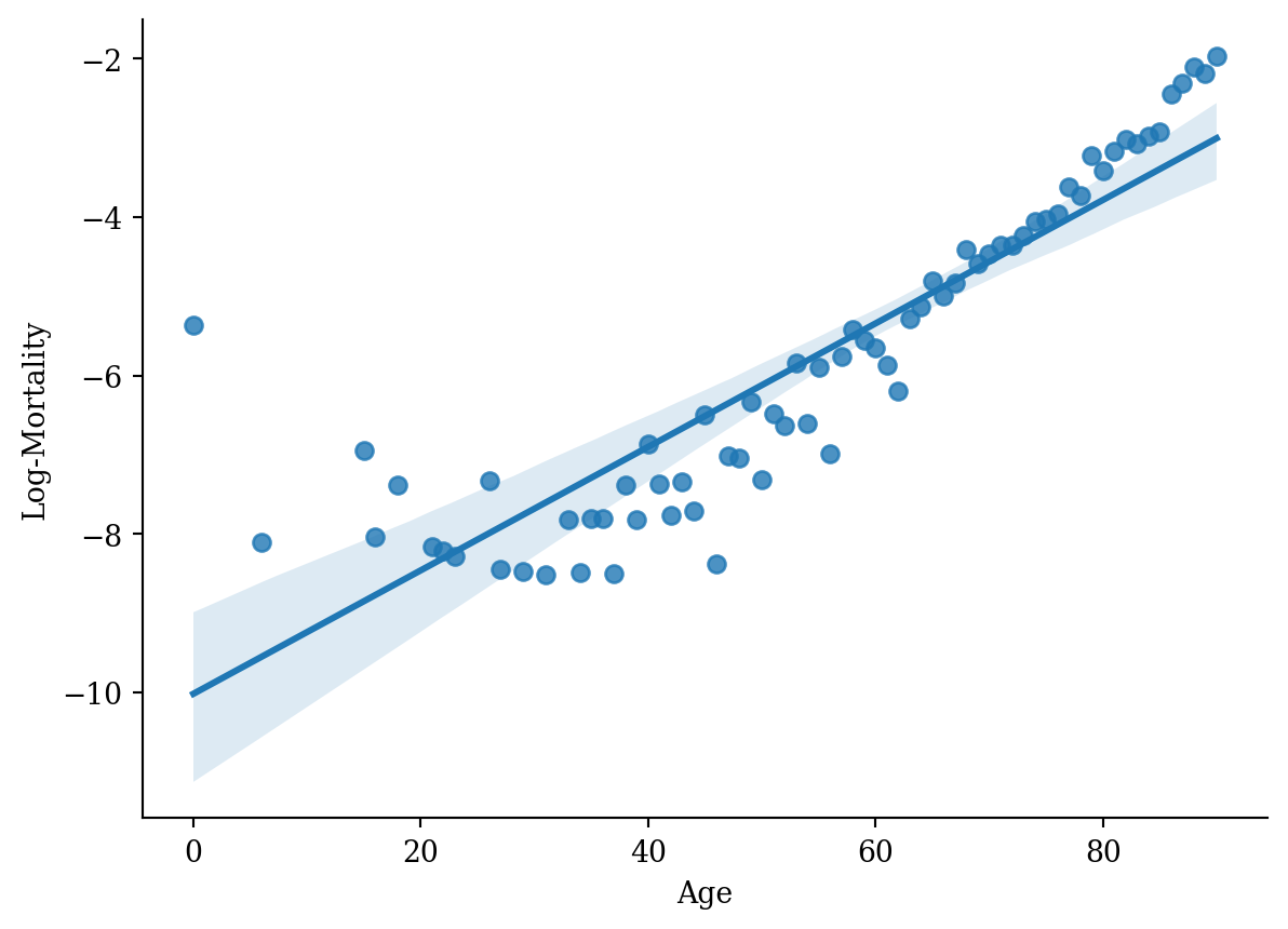

Interpolating

R

df_grid <- data.frame(age = seq(25, 35, by = 0.5))
df_grid$log_mx <- predict(model_lr, newdata = df_grid)

lux_young <- lux_2020 %>% filter(age >= 25, age <= 35)

ggplot(lux_young, aes(x = age, y = log_mx)) + 
  theme_minimal() +
  geom_point(data = df_grid, aes(y = log_mx), color = "red", size = 2) +
  geom_point(alpha = 0.75, size = 2) +
  labs(x = "Age", y = "Log-Mortality")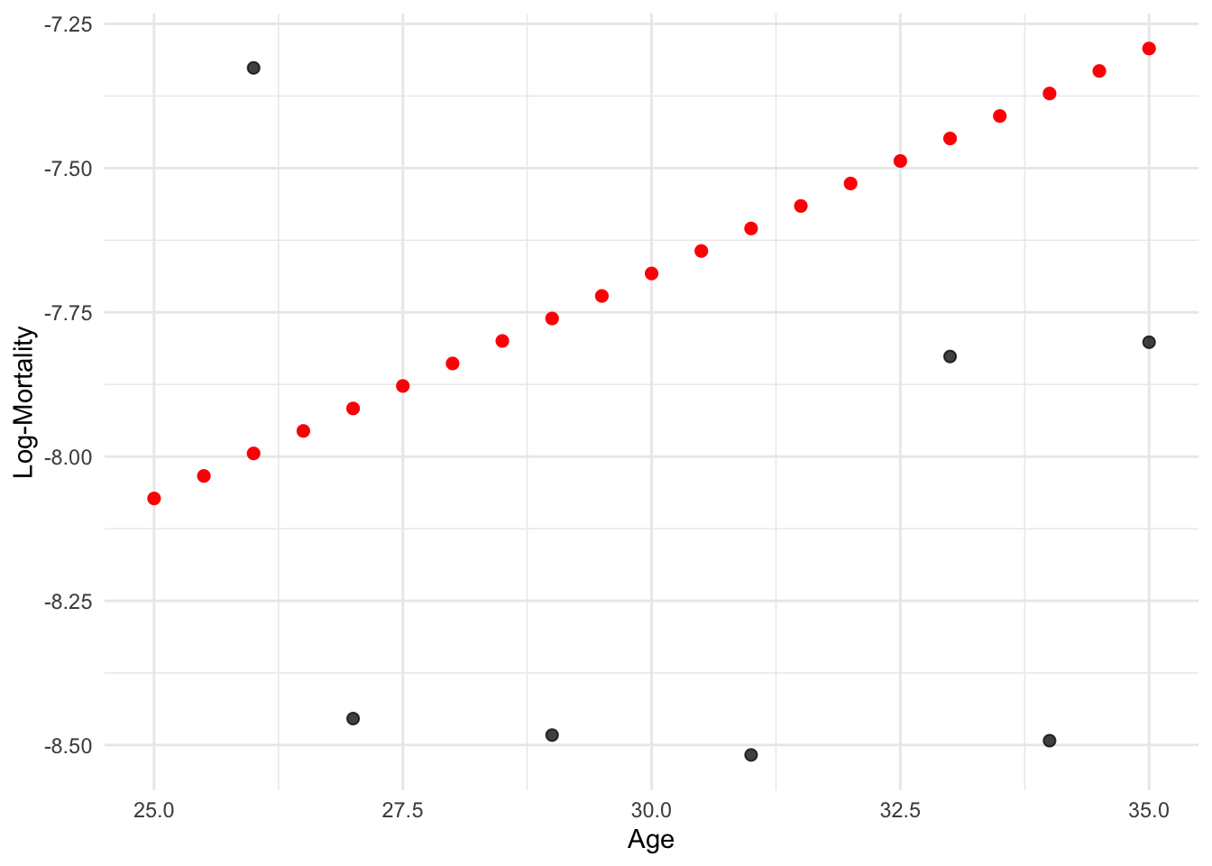

Python

age_grid = pd.DataFrame({"age": np.arange(25, 35, 0.5)})
predictions = model.predict(age_grid)

lux_young = lux_2020[(lux_2020['age'] >= 25) & (lux_2020['age'] <= 35)] 
plt.scatter(lux_young['age'], lux_young['log_mx'], alpha=0.75)
plt.scatter(age_grid, model.predict(age_grid), color='red', marker='o')
plt.xlabel('Age'); plt.ylabel('Log-Mortality');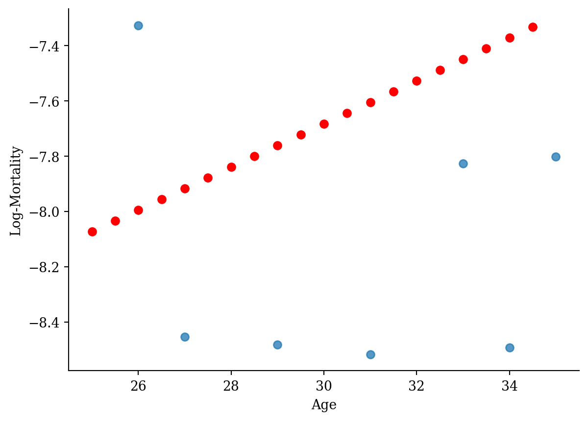

Extrapolating

R

df_grid <- data.frame(age = seq(40, 130))
df_grid$log_mx <- predict(model_lr, newdata = df_grid)

lux_old <- lux_2020 %>% filter(age >= 40, age <= 130)

ggplot(lux_old, aes(x = age, y = log_mx)) + 
  theme_minimal() +
  geom_line(data = df_grid, aes(y = log_mx), color = "red", linewidth = 2) +
  geom_point(alpha = 0.75) +
  labs(x = "Age", y = "Log-Mortality")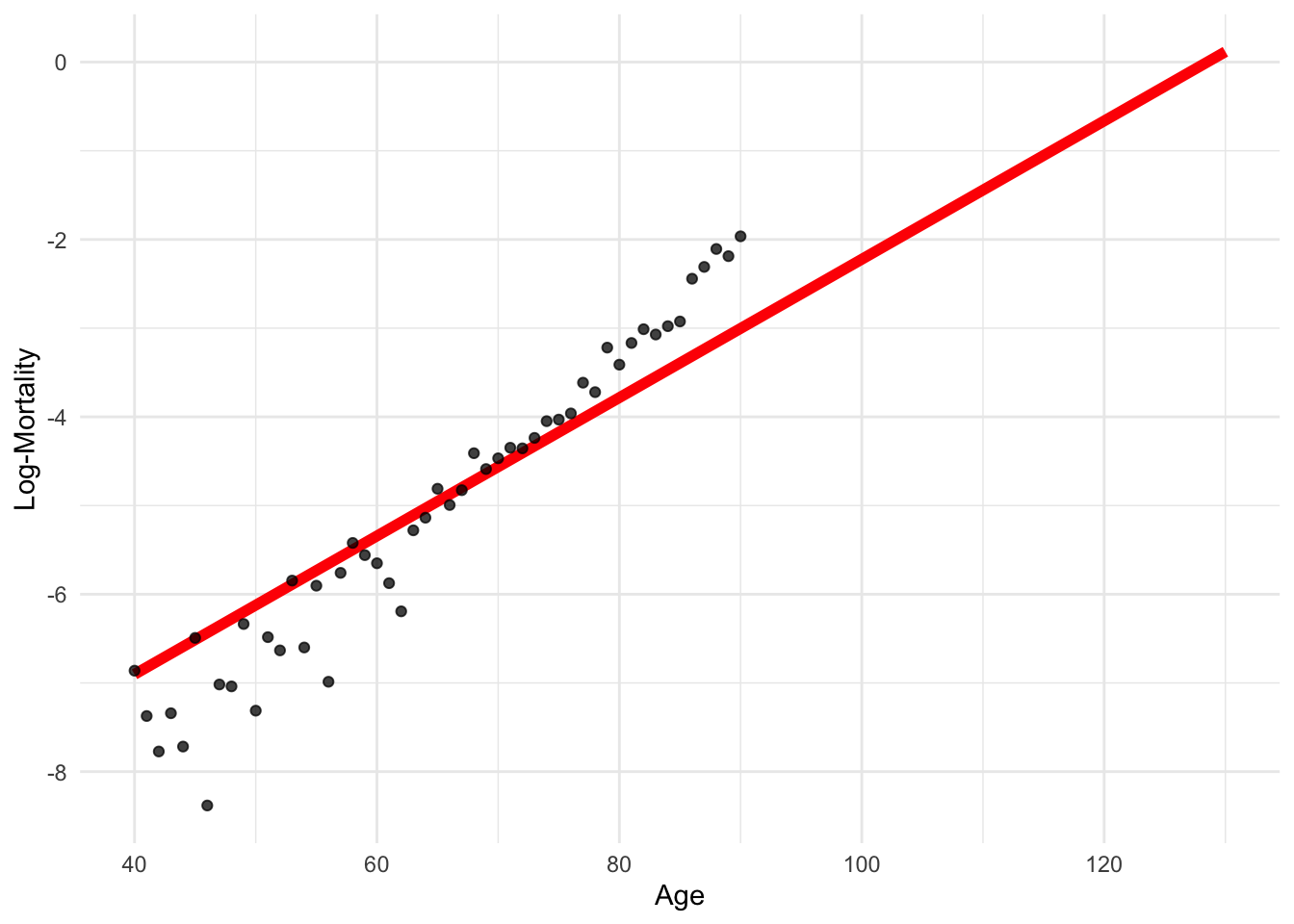

Python

age_grid = pd.DataFrame({"age": np.arange(40, 130)})
predictions = model.predict(age_grid)

lux_old = lux_2020[(lux_2020['age'] >= 40) & (lux_2020['age'] <= 130)] 
plt.plot(age_grid, model.predict(age_grid), color='red', marker='o')
plt.scatter(lux_old['age'], lux_old['log_mx'], alpha=0.75)
plt.xlabel('Age'); plt.ylabel('Log-Mortality');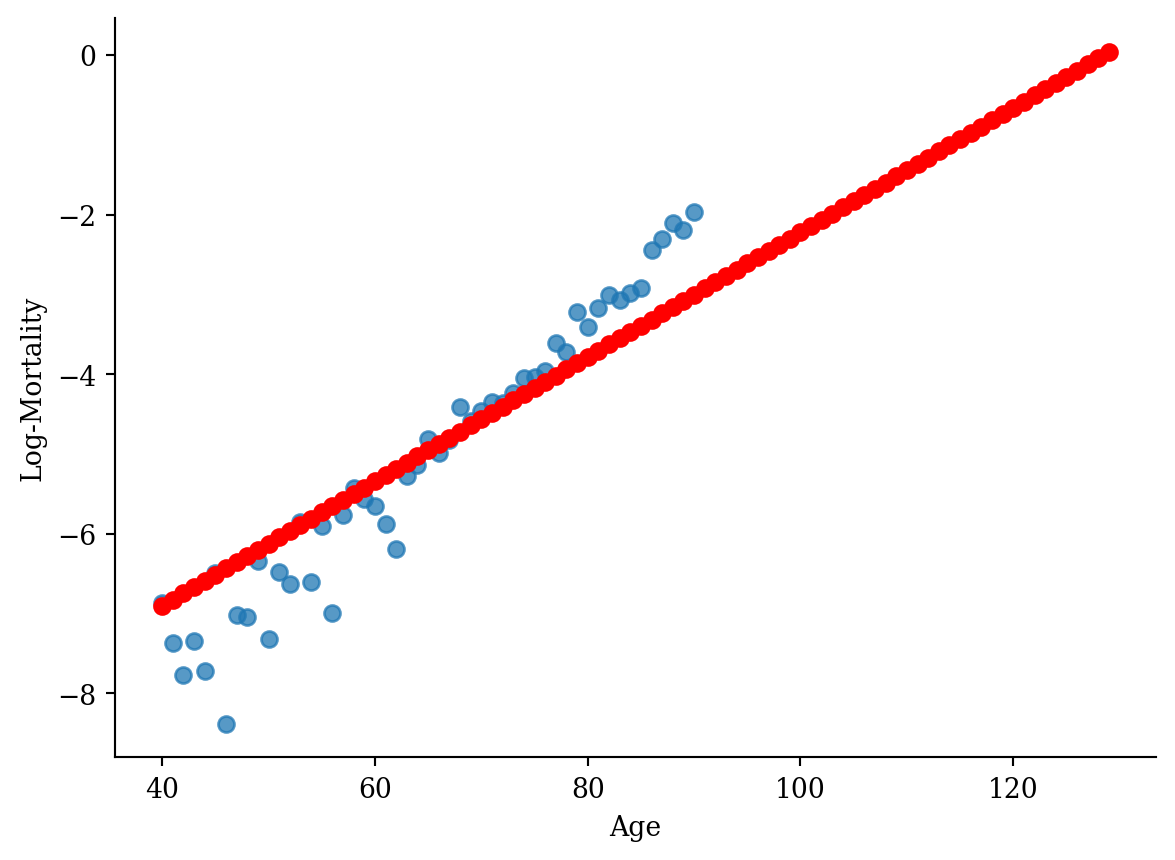

Multiple linear regression

df_mlr = lux[c("age", "year", "log_mx")]
head(df_mlr)

# A tibble: 6 × 3
    age  year log_mx
  <int> <int>  <dbl>
1     0  1960  -3.74
2     1  1960  -6.38
3     2  1960  -6.37
4     3  1960  -6.68
5     4  1960  -7.08
6     5  1960  -7.04

Fitting:

linear_model <- lm(log_mx ~ age + year, data = df_mlr)

Predicting:

new_point <- data.frame(year = 2040, age = 20)
predict(linear_model, newdata = new_point)

    1 
-8.66 

coef(linear_model)

(Intercept)         age        year 
34.58222358  0.07287039 -0.02191158 

Fitted multiple linear regression

# This code chunk is courtesy of ChatGPT.
library(plotly)
model <- lm(log_mx ~ age + year, data = lux)
# Predict values over a grid to create the regression plane
# Create a sequence of ages and years that covers the range of your data
age_range <- seq(min(lux$age), max(lux$age), length.out = 100)
year_range <- seq(min(lux$year), max(lux$year), length.out = 100)

# Create a grid of age and year values
grid <- expand.grid(age = age_range, year = year_range)

# Predict log_mx for the grid
grid$log_mx <- predict(model, newdata = grid)

# Plot
fig <- plot_ly(lux, x = ~age, y = ~year, z = ~log_mx, type = 'scatter3d', mode = 'markers', size = 0.5) %>%
  add_trace(data = grid, x = ~age, y = ~year, z = ~log_mx, type = 'mesh3d', opacity = 0.5) %>%
  layout(scene = list(xaxis = list(title = 'Age'),
                      yaxis = list(title = 'Year'),
                      zaxis = list(title = 'Log-Mortality')))

# Show the plot
fig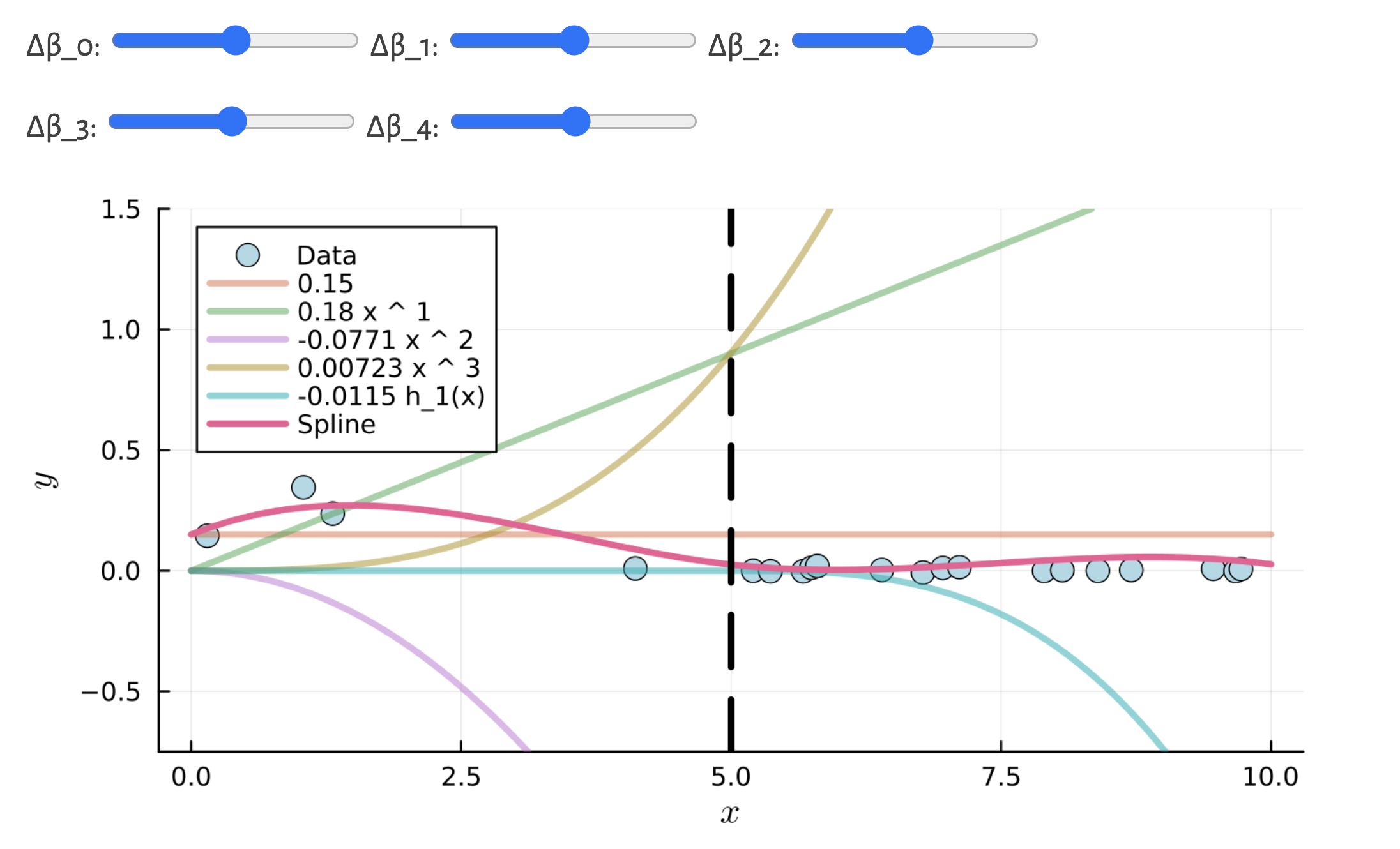

Link to interactive notebook

See the spline demo notebook for a high-level view of these methods

Polynomial Regression

Polynomial regression

Extend the standard linear model

y_i = \beta_0 + \beta_1 x_i + \varepsilon_i

to

y_i = \beta_0 + \beta_1 x_i + \beta_2 x_i^2 + \cdots + \beta_d x_i^d + \varepsilon_i

• Relaxes the assumption that predictor and response are linearly related.
• Works almost identically to multiple linear regression, except the other “predictors” are just transformations of the initial predictor.

Quadratic regression (by hand)

df_pr <- data.frame(age = lux_2020$age, age2 = lux_2020$age^2, log_mx = lux_2020$log_mx)
head(df_pr)

  age age2    log_mx
1   0    0 -5.363176
2   6   36 -8.111728
3  15  225 -6.949619
4  16  256 -8.040959
5  18  324 -7.389022
6  21  441 -8.159519

manual_poly_model <- lm(log_mx ~ age + age2,
    data = df_pr)
coef(manual_poly_model)

 (Intercept)          age         age2 
-7.065977594 -0.066603952  0.001421058 

impossible_x <- data.frame(age=20, age2=20)
predict(manual_poly_model, newdata = impossible_x)

        1 
-8.369635 

ggplot(lux_2020, aes(x = age, y = log_mx)) + theme_minimal() +
  geom_line(data = df_pr, aes(x = age, y = predict(manual_poly_model)), color = "red", linewidth=2) +
  geom_point(alpha = 0.75) + labs(x = "Age", y = "Log-Mortality")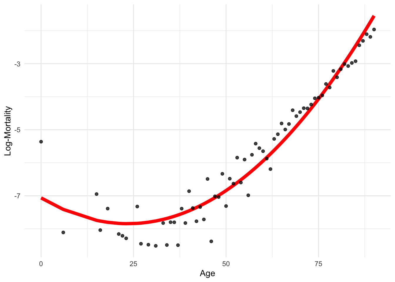

We “tricked” into thinking that age2 is a separate variable!

This is a linear model of a nonlinearly transformed variable.

The poly function

df_pr <- data.frame(age = lux_2020$age, log_mx = lux_2020$log_mx)
head(df_pr)

  age    log_mx
1   0 -5.363176
2   6 -8.111728
3  15 -6.949619
4  16 -8.040959
5  18 -7.389022
6  21 -8.159519

poly_model <- lm(log_mx ~ poly(age, 2),
    data = df_pr)
coef(poly_model)

  (Intercept) poly(age, 2)1 poly(age, 2)2 
    -5.787494     14.534731      6.376355 

Now we can’t put in age^2 as a separate variable.

new_input <- data.frame(age = 20)
predict(poly_model, newdata = new_input)

        1 
-7.829633 

ggplot(lux_2020, aes(x = age, y = log_mx)) + theme_minimal() +
  geom_line(data = df_pr, aes(x = age, y = predict(poly_model)), color = "red", linewidth=2) +
  geom_point(alpha = 0.75) + labs(x = "Age", y = "Log-Mortality")

Note

The coefficients are different, but the predictions are the same!

Quadratic regression with error bars

ggplot(lux_2020, aes(x = age, y = log_mx)) + theme_minimal() +
  stat_smooth(method = "lm", formula = y ~ poly(x, 2), color = "red", linewidth=2) +
  geom_point(alpha = 0.75) + labs(x = "Age", y = "Log-Mortality")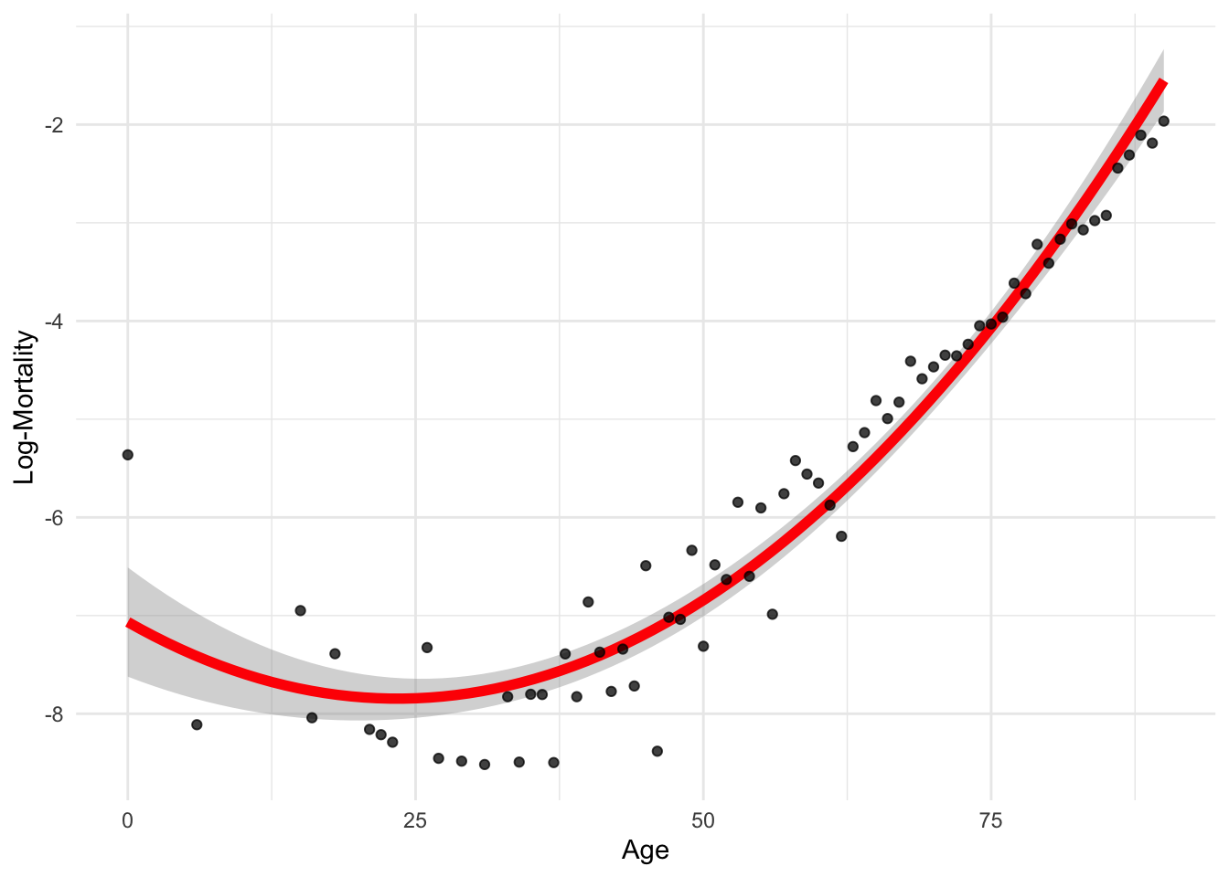

Polynomial expansion

head(lux$age)

[1] 0 1 2 3 4 5

age_poly <- model.matrix(~ poly(age, 2), data = lux)
head(age_poly)

  (Intercept) poly(age, 2)1 poly(age, 2)2
1           1   -0.03020513    0.03969719
2           1   -0.02961226    0.03744658
3           1   -0.02901939    0.03524373
4           1   -0.02842652    0.03308866
5           1   -0.02783365    0.03098136
6           1   -0.02724077    0.02892183

age_poly <- model.matrix(~ poly(age, 2, raw=TRUE), data = lux)
head(age_poly)

  (Intercept) poly(age, 2, raw = TRUE)1 poly(age, 2, raw = TRUE)2
1           1                         0                         0
2           1                         1                         1
3           1                         2                         4
4           1                         3                         9
5           1                         4                        16
6           1                         5                        25

Monomials plotted (raw=TRUE)

age_poly <- model.matrix(~ poly(age, 2, raw=TRUE), data = lux)

df_poly <- data.frame(age = lux$age, age_poly[, -1])

df_poly_long <- df_poly %>%
  pivot_longer(cols = -age, names_to = "Polynomial", values_to = "Value")

ggplot(df_poly_long, aes(x = age, y = Value, color = Polynomial)) +
  geom_line(linewidth=2) +
  theme_minimal() +
  labs(title = "Polynomial Terms of Age",
       x = "Age",
       y = "Polynomial Value",
       color = "Term")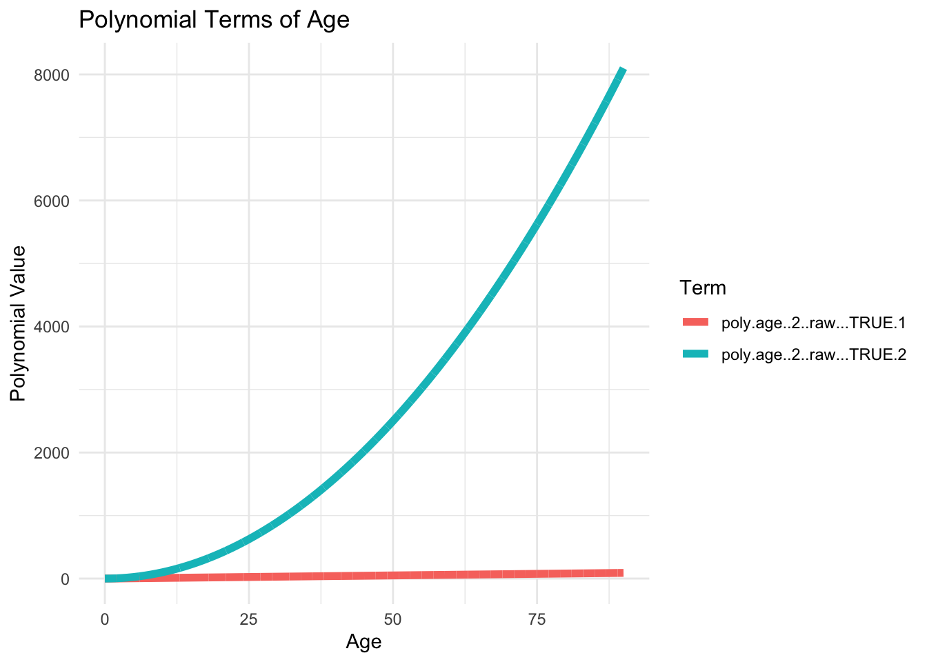

Orthogonal polynomials plotted (default)

age_poly <- model.matrix(~ poly(age, 4), data = lux)

df_poly <- data.frame(age = lux$age, age_poly[, -1])

df_poly_long <- df_poly %>%
  pivot_longer(cols = -age, names_to = "Polynomial", values_to = "Value")

ggplot(df_poly_long, aes(x = age, y = Value, color = Polynomial)) +
  geom_line(linewidth=2) +
  theme_minimal() +
  labs(title = "Polynomial Terms of Age",
       x = "Age",
       y = "Polynomial Value",
       color = "Term")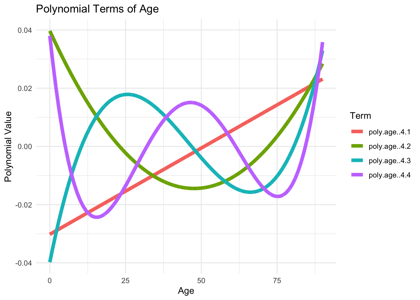

Why? Raw polynomials can be highly correlated

Reciprocal of the condition number is rcond.

X <- model.matrix(~ poly(age, 10),
    data = lux)
rcond(t(X) %*% X)

[1] 0.0002087683

X_raw <- model.matrix(~ poly(age, 10, raw=TRUE),
    data = lux)
rcond(t(X_raw) %*% X_raw)

[1] 1.153253e-40

If this number is (very) close to 0, the computer will have a hard time finding the inverse of the matrix.

inv <- solve(t(X) %*% X)

inv <- solve(t(X_raw) %*% X_raw)

Error in solve.default(t(X_raw) %*% X_raw): system is computationally singular: reciprocal condition number = 1.15325e-40

Summaries of the two models

Can you spot an important difference?

summary(manual_poly_model)

Call:
lm(formula = log_mx ~ age + age2, data = df_pr)

Residuals:
     Min       1Q   Median       3Q      Max 
-1.25899 -0.33912 -0.03671  0.30503  1.70280 

Coefficients:
              Estimate Std. Error t value Pr(>|t|)    
(Intercept) -7.0659776  0.2787615 -25.348  < 2e-16 ***
age         -0.0666040  0.0115898  -5.747 2.43e-07 ***
age2         0.0014211  0.0001108  12.820  < 2e-16 ***
---
Signif. codes:  0 '***' 0.001 '**' 0.01 '*' 0.05 '.' 0.1 ' ' 1

Residual standard error: 0.4974 on 67 degrees of freedom
Multiple R-squared:  0.9383,    Adjusted R-squared:  0.9364 
F-statistic: 509.2 on 2 and 67 DF,  p-value: < 2.2e-16

summary(poly_model)

Call:
lm(formula = log_mx ~ poly(age, 2), data = df_pr)

Residuals:
     Min       1Q   Median       3Q      Max 
-1.25899 -0.33912 -0.03671  0.30503  1.70280 

Coefficients:
              Estimate Std. Error t value Pr(>|t|)    
(Intercept)   -5.78749    0.05945  -97.36   <2e-16 ***
poly(age, 2)1 14.53473    0.49736   29.22   <2e-16 ***
poly(age, 2)2  6.37636    0.49736   12.82   <2e-16 ***
---
Signif. codes:  0 '***' 0.001 '**' 0.01 '*' 0.05 '.' 0.1 ' ' 1

Residual standard error: 0.4974 on 67 degrees of freedom
Multiple R-squared:  0.9383,    Adjusted R-squared:  0.9364 
F-statistic: 509.2 on 2 and 67 DF,  p-value: < 2.2e-16

Polynomial regression: increasing the order

orders <- 1:20
for (i in seq_along(orders)) {
  order <- orders[i]

  formula <- as.formula(glue("log_mx ~ poly(age, {order})"))
  model <- lm(formula, data = lux_2020)
  
  age_grid$log_mx <- predict(model, newdata = age_grid)
  
  plot_regression(lux_2020, age_grid, "age", "log_mx",
                  glue("Polynomial Regression Order {order}"), 
                  glue("./Animations/NonLinear/Poly{i}.svg"))
}

Can easily use polynomials in classification

(Right Side:) Model of binary event Wage > 250 via logistic regression

\mathbb{P}(y_i > 250|x_i) = \frac{\exp(\beta_0 + \beta_1x_i + \beta_2x_i^2 + \beta_3x_i^3 + \beta_4x_i^4)}{1+\exp(\beta_0 + \beta_1x_i + \beta_2x_i^2 + \beta_3x_i^3 + \beta_4x_i^4)}

Source: James et al. (2021), An Introduction to Statistical Learning with Applications in R, Figure 7.1.

Polynomial regression: notes and problems

Pros:

• Can model more complex relationships.
• Can also be used in logistic regression, or any linear-like regression for that matter.

Cons:

• Usually one sticks to polynomials of degree 2-4; shape can get very erratic with higher degrees.
• Can be computationally unstable with high degrees.
• Can be difficult to interpret.

Step Functions

Step functions

• Polynomial regression imposes a global structure on the nonlinear function; a simple alternative is to use step functions.

• Break up the range of x into k+1 distinct regions (or “bins”), using k cutpoints: c_1 < c_2 < \dots < c_k

• Do a least squares fit on y_i = \beta_0 + \beta_1 I(c_1 \leq x_i < c_2) + \beta_2 I(c_2 \leq x_i < c_3) + \dots + \beta_{k-1} I(c_{k-1} \leq x_i < c_k) + \beta_k I(c_k \leq x_i)

Example: Step functions

Step function regression on Wage data

Same Wage example as before but with step functions.

Source: James et al. (2021), An Introduction to Statistical Learning with Applications in R, Figure 7.2.

Using I and cut

head(model.matrix(~ age + I(age >= 3), data = lux))

  (Intercept) age I(age >= 3)TRUE
1           1   0               0
2           1   1               0
3           1   2               0
4           1   3               1
5           1   4               1
6           1   5               1

head(cut(lux$age, breaks=c(0, 5, 100), right=T))

[1] <NA>  (0,5] (0,5] (0,5] (0,5] (0,5]
Levels: (0,5] (5,100]

head(model.matrix(~ age + cut(age, breaks=c(0, 5, 100), right=T), data = lux))

  (Intercept) age cut(age, breaks = c(0, 5, 100), right = T)(5,100]
2           1   1                                                 0
3           1   2                                                 0
4           1   3                                                 0
5           1   4                                                 0
6           1   5                                                 0
7           1   6                                                 1

model_step <- lm(log_mx ~ cut(age, breaks=c(0, 5, 100), right=T), data = lux)
coef(model_step)

                                      (Intercept) 
                                        -7.253560 
cut(age, breaks = c(0, 5, 100), right = T)(5,100] 
                                         2.011324 

Letting breaks be a single number

head(cut(lux$age, breaks=4, right=T))

[1] (-0.09,22.5] (-0.09,22.5] (-0.09,22.5] (-0.09,22.5] (-0.09,22.5]
[6] (-0.09,22.5]
Levels: (-0.09,22.5] (22.5,45] (45,67.5] (67.5,90.1]

model_step <- lm(log_mx ~ cut(age, breaks=4, right=T), data = lux)
summary(model_step)

Call:
lm(formula = log_mx ~ cut(age, breaks = 4, right = T), data = lux)

Residuals:
    Min      1Q  Median      3Q     Max 
-3.1872 -0.6035 -0.0220  0.5886  3.5764 

Coefficients:
                                           Estimate Std. Error  t value
(Intercept)                                -7.24326    0.03111 -232.817
cut(age, breaks = 4, right = T)(22.5,45]    0.14673    0.03896    3.766
cut(age, breaks = 4, right = T)(45,67.5]    1.98093    0.03825   51.783
cut(age, breaks = 4, right = T)(67.5,90.1]  4.37103    0.03797  115.126
                                           Pr(>|t|)    
(Intercept)                                 < 2e-16 ***
cut(age, breaks = 4, right = T)(22.5,45]   0.000168 ***
cut(age, breaks = 4, right = T)(45,67.5]    < 2e-16 ***
cut(age, breaks = 4, right = T)(67.5,90.1]  < 2e-16 ***
---
Signif. codes:  0 '***' 0.001 '**' 0.01 '*' 0.05 '.' 0.1 ' ' 1

Residual standard error: 0.8284 on 4786 degrees of freedom
Multiple R-squared:  0.8227,    Adjusted R-squared:  0.8226 
F-statistic:  7404 on 3 and 4786 DF,  p-value: < 2.2e-16

More general viewpoint: Basis functions

Fit the model:

y_i = \beta_0 + \beta_1 b_1(x_i) + \beta_2 b_2(x_i) + \dots + \beta_k b_k(x_i)

• b_1(x_i), b_2(x_i), \dots, b_k(x_i) are “basis functions”.
• Transform the predictor before fitting, yielding multiple derived “predictors”.

\boldsymbol{X} = \begin{bmatrix} 1 & x_{11} & x_{12} & \dots & x_{1p} \\ 1 & x_{21} & x_{22} & \dots & x_{2p} \\ \vdots & \vdots & \vdots & \ddots & \vdots \\ 1 & x_{n1} & x_{n2} & \dots & x_{np} \end{bmatrix}

\boldsymbol{X} = \begin{bmatrix} 1 & b_1(x_1) & b_2(x_1) & \dots & b_k(x_1) \\ 1 & b_1(x_2) & b_2(x_2) & \dots & b_k(x_2) \\ \vdots & \vdots & \vdots & \ddots & \vdots \\ 1 & b_1(x_n) & b_2(x_n) & \dots & b_k(x_n) \end{bmatrix}

• For polynomial regression, b_j(x_i) = x_i^j
• For step function regression, b_j(x_i) = I(c_j \leq x_i < c_{j+1}) if j=1,\dots,k-1

Regression Splines

Why not both?

• We can combine the previous two ideas (polynomial regression and step functions) to gain flexibility.

• For example, you could fit a piecewise cubic polynomial with one “knot”: y_i = \begin{cases} \beta_{0,1} + \beta_{1,1} x_i + \beta_{2,1} x_i^2 + \beta_{3,1} x_i^3 & \text{ if } x_i < c \\ \beta_{0,2} + \beta_{1,2} x_i + \beta_{2,2} x_i^2 + \beta_{3,2} x_i^3 & \text{ if } x_i \geq c \end{cases}

• We call c a “knot”: a point of our choosing where the coefficients of the model change.

• Question: what are possible issues with this approach?

Unconstrained cubic regression

Unconstrained cubic regression on Wage data

Spline definition

A piecewise polynomial function of degree d is a spline if the function is continuous up to its (d-1)th derivative at each knot.

• A 1st degree spline is a piecewise linear function which is continuous. I.e., we require the 0th derivative (which is the function itself) to be continuous (so, “step functions” are not allowed).
• A 2nd degree spline is a piecewise quadratic function which is continuous and has a continuous derivative.
• A 3rd degree spline is a piecewise cubic function which is continuous and has continuous 1st and 2nd derivatives.

Example: Linear spline

model <- lm(log_mx ~ bs(age, degree=1, knots=...), data = lux_2020)

# Linear regression splines with different number of knots
knots_seq <- 2:11
for (i in seq_along(knots_seq)) {
  n_knots <- knots_seq[i]
  knots <- quantile(lux_2020$age, probs = seq(0, 1, length.out = n_knots + 1))[-c(1, n_knots + 2)]
  formula <- as.formula(glue("log_mx ~ bs(age, degree=1, knots = c({toString(knots)}))"))
  model <- lm(formula, data = lux_2020)
  
  age_grid$log_mx <- predict(model, newdata = age_grid)
  
  plot_regression(lux_2020, age_grid, "age", "log_mx",
                  glue("Cubic Spline with {n_knots} Knots"), 
                  glue("./Animations/NonLinear/SplineCub{i}.svg"),
                  knots = knots)
}

Example: Cubic spline

model <- lm(log_mx ~ bs(age, degree=3, knots=...), data = lux_2020)

# Cubic regression splines with different number of knots
knots_seq <- 2:11
for (i in seq_along(knots_seq)) {
  n_knots <- knots_seq[i]
  knots <- quantile(lux_2020$age, probs = seq(0, 1, length.out = n_knots + 1))[-c(1, n_knots + 2)]
  formula <- as.formula(glue("log_mx ~ bs(age, degree=3, knots = c({toString(knots)}))"))
  model <- lm(formula, data = lux_2020)
  
  age_grid$log_mx <- predict(model, newdata = age_grid)
  
  plot_regression(lux_2020, age_grid, "age", "log_mx",
                  glue("Cubic Spline with {n_knots} Knots"), 
                  glue("./Animations/NonLinear/SplineCub{i}.svg"),
                  knots = knots)
}

Examples: Different types of splines

Four varieties of splines fit on a subset of the Wage data

Source: James et al. (2021), An Introduction to Statistical Learning with Applications in R, Figure 7.3.

Cubic splines & natural splines

• The cubic is preferred as it is the smallest order where the knots are not visible without close inspection.

• We can extend the idea of a cubic spline to a natural cubic spline. It is a spline where outside the boundary knots (extrapolation) the function is linear.

Cubic spline & natural cubic spline fit to Wage subset

Degree-15 spline & natural cubic spline fit to Wage data

Source: James et al. (2021), An Introduction to Statistical Learning with Applications in R, Figures 7.4 and 7.7.

Smoothing Splines

Smoothing splines

• Goal: fit a function g which minimises the MSE whilst still being ‘smooth’, i.e.,

\text{minimise:} \quad \frac{1}{n} \sum_{i=1}^n (y_i - g(x_i))^2 + \lambda \int g''(x)^2 \, \mathrm{d}x.

• The integral term is a penalty on the “roughness” of g, with \lambda a tuning parameter (larger \lambda means we penalise more a rough fit).
• \lambda = 0: g will be very lumpy and will just interpolate all training data points (more flexible: less bias for more variance).
• \lambda \to \infty: g will be a straight line fit (less flexible: more bias for less variance).
• The solution for g turns out to be a (shrunken) natural cubic spline, with knots at every training data point.

Note

For mortality smoothing, US uses smoothing splines, UK uses regression splines.

Example: Smoothing splines

model <- smooth.spline(lux_2020$age, lux_2020$log_mx, df = df)

# Smoothing splines with different df (degrees of freedom)
dfs <- seq(2, 20, length.out = 10)

for (i in seq_along(dfs)) {
  df <- dfs[i]
  model <- smooth.spline(lux_2020$age, lux_2020$log_mx, df = df)
  predictions <- predict(model, age_grid$age)
  age_grid$log_mx <- predictions$y
  
  plot_regression(lux_2020, age_grid, "age", "log_mx",
                  glue("Smoothing Spline with df {df}"), 
                  glue("./Animations/NonLinear/SmoothSpline{i}.svg"))
}

Choosing \lambda

• The smaller the \lambda, the more flexible (but rougher) the fit is.
• The “effective degrees of freedom” (denoted df_\lambda) of our model hence depend on \lambda.
  • df_\lambda measures the flexibility of the smoothing spline.
  • it can be a non-integer (since some coefficients are constrained, they are not completely free to vary).
• Choice of \lambda can be done via Cross validation.
• LOOCV error can be computed using only one computation for each \lambda; extremely computationally efficient.
• Note a good thing about smoothing splines (in comparison to regression splines) is that we do not have to pick the “degree” of the polynomial, nor the location of our knots.

Choosing \lambda for the Luxembourg mortality data

cv.spline <- smooth.spline(lux_2020$age, lux_2020$log_mx, cv=TRUE)
cv.spline$df

[1] 5.08017

plot(lux_2020$age, lux_2020$log_mx, xlab="age", ylab="log_mx", pch=19)
lines(cv.spline, col="brown3", lwd=3)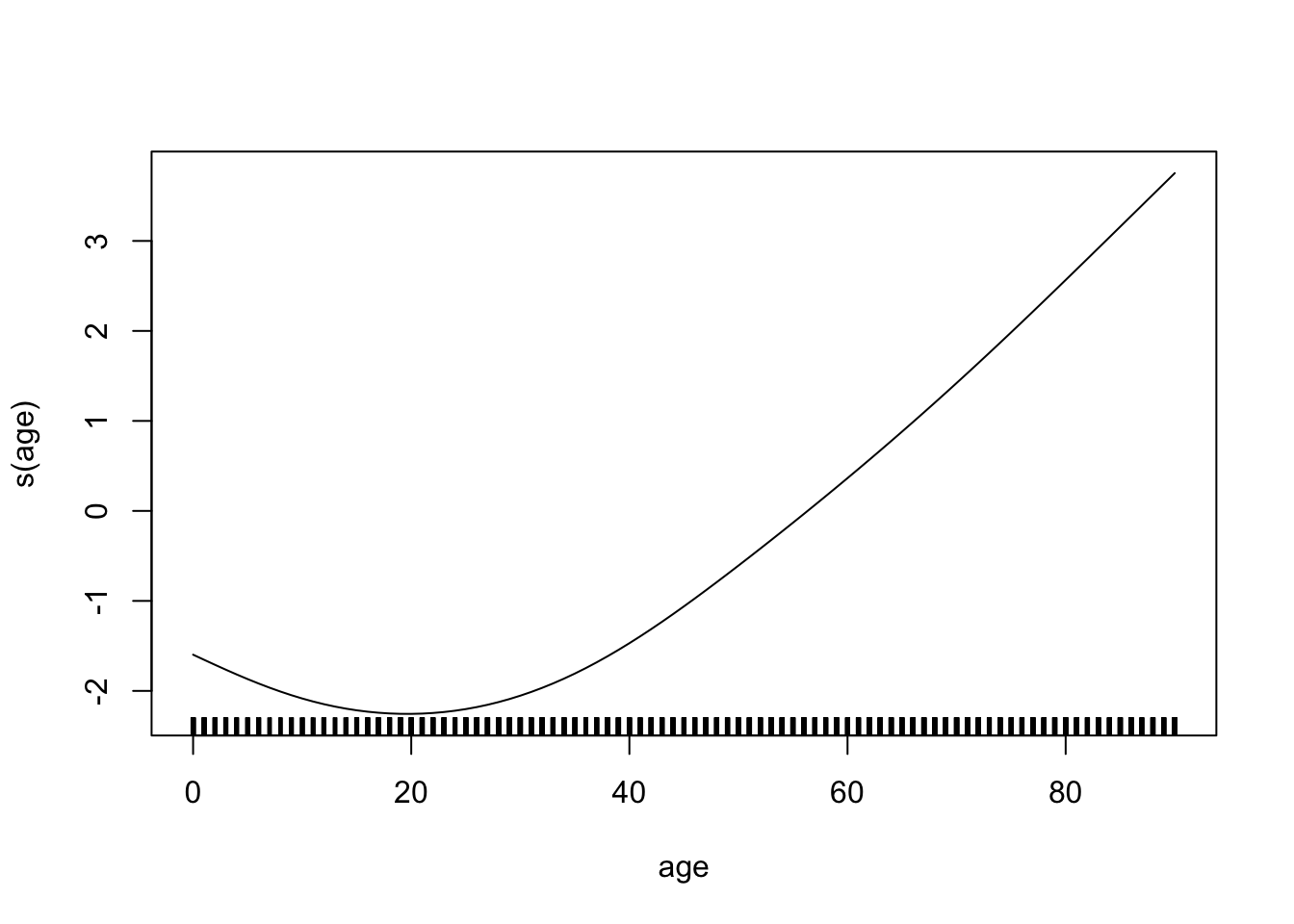

Smoothing splines on Wage data

Comparing smoothing splines

Source: James et al. (2021), An Introduction to Statistical Learning with Applications in R, Figure 7.8.

Local Regression

Local regression

• Idea: predict the response y_0 associated with predictor x_0 via a linear fit, but using only the data points (x_i,y_i) that are “close” to x_0.

• Algorithm:

  1. Gather the fraction s = k/n of training points that are the closest to x_0 (in their x_i values).
  2. Assign each a weight K_{i0} = K(x_i, x_0), based on how close they are to x_0 (closer points get a higher weight). Points outside those k nearest neighbours get a weight of 0.
  3. Fit weighted least squares regression of the y_i on the x_i, by minimising \sum_{i=1}^n K_{i0}(y_i - \beta_0 - \beta_1x_i)^2
  4. The fitted value is then \hat{y}_0=\hat{f}(x_0) = \hat{\beta}_0 + \hat{\beta}_1x_0.

Local regression example

Example of making predictions with local regression at x \approx 0.05 and x \approx 0.45

Source: James et al. (2021), An Introduction to Statistical Learning with Applications in R, Figure 7.9.

Local regression: comments

• Local regression does a weighted regression, using only the points around a given x_0.
• We don’t obtain a “global” equation of best fit: we need to run the procedure for each point x_0 at which we want a fitted y_0.
• Useful for updating models to recently obtained data.
• Possible to extend this idea to a few predictors (2,3, maybe 4): just have the weights based on distance in 2D, 3D or 4D space.
• Things can get problematic when p > 4, as there will be very few (if any) training observations in the neighbourhood of most points.

Local regression on Wage data

You can adjust the smoothness by changing the span

Source: James et al. (2021), An Introduction to Statistical Learning with Applications in R, Figure 7.10.

Generalised Additive Models (GAMs)

Generalised Additive Models: GAMs

• We can tranform several predictors in a non-linear way, and put them together in one model to predict y_i (as in multiple linear regression):

y_i = \beta_0 + f_1(x_{i,1}) + f_2(x_{i,2}) + ... + f_p(x_{i,p}) + \varepsilon_i

• The f_j can be virtually any function of the predictors, but all those discussed earlier (polynomials, step functions, regression and smoothing splines) are common choices.
• We can find a separate f_j for each predictor, and then just add them together in our model.
• Note we preserve the additive property of individual effects.
• Can also be used on categorical responses in a logistic regression setting.

Example: GAM on Wage data

GAM fit using regression splines

• Each plot shows the contribution of each predictor to wage.
• education is qualitative. The others are fit with natural cubic splines.

Source: James et al. (2021), An Introduction to Statistical Learning with Applications in R, Figure 7.11.

Example: GAM on Wage data

GAM fit using smoothing splines

• Each plot shows the contribution of each predictor to wage.
• education is qualitative. The others are fit with smoothing splines.

Source: James et al. (2021), An Introduction to Statistical Learning with Applications in R, Figure 7.12.

GAMs: pros and cons

• GAMs allow us to consider nonlinear relationships between the predictors and response, which can give a better fit.
• Model is additive: we can still interpret the effect of individual predictors on the response.
• However, model additivity potentially ignores interaction effects between predictors. That said, one could always add two-dimensional functions f_{j,k}(x_j, x_k) in the model, which depend on two preditors in a “non-additive” way.

GAMs on Luxembourg data (using mgcv package)

library(mgcv)
model_gam <- gam(log_mx ~ s(age) + s(year), data=lux)

plot(model_gam, select=1)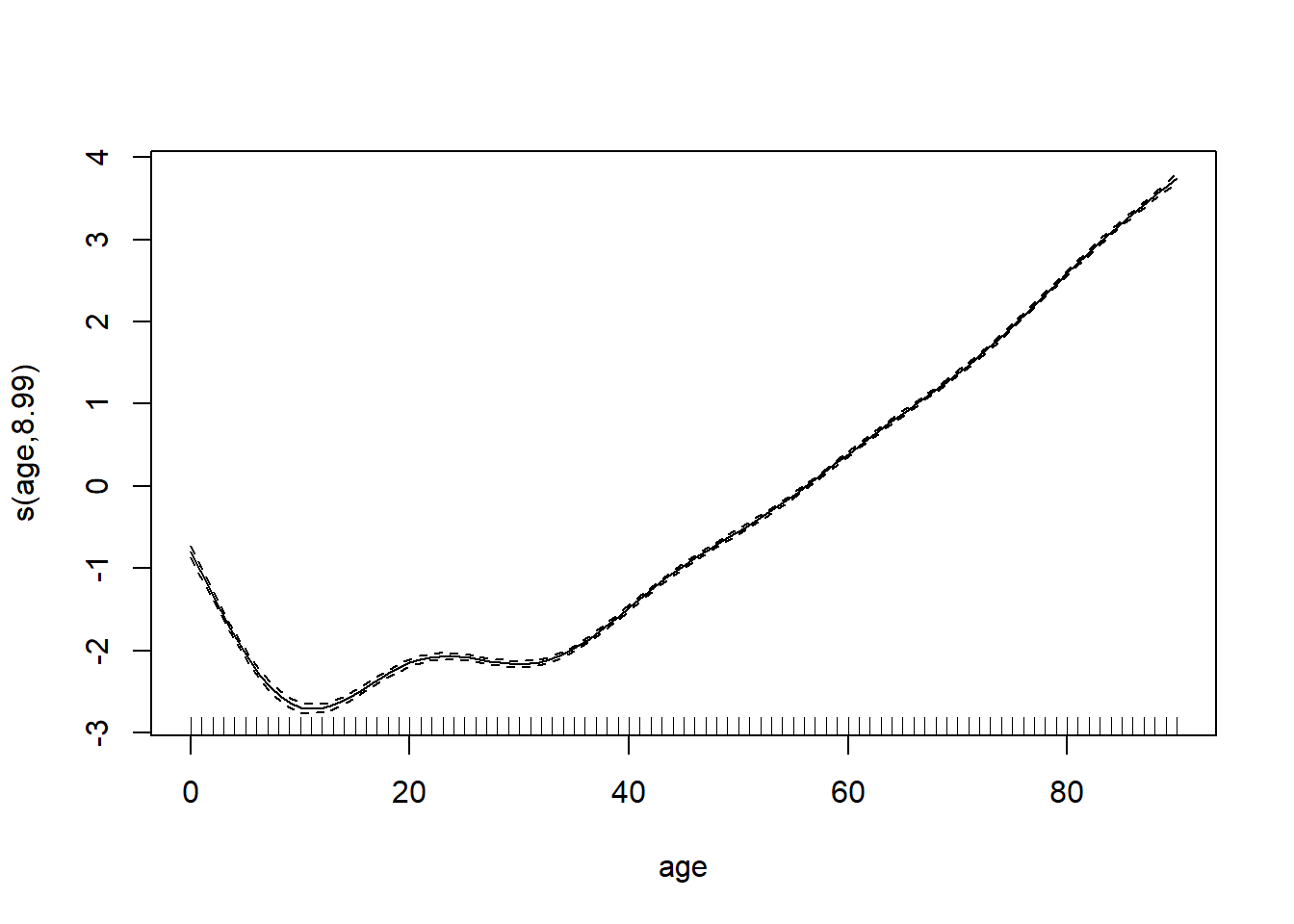

plot(model_gam, select=2)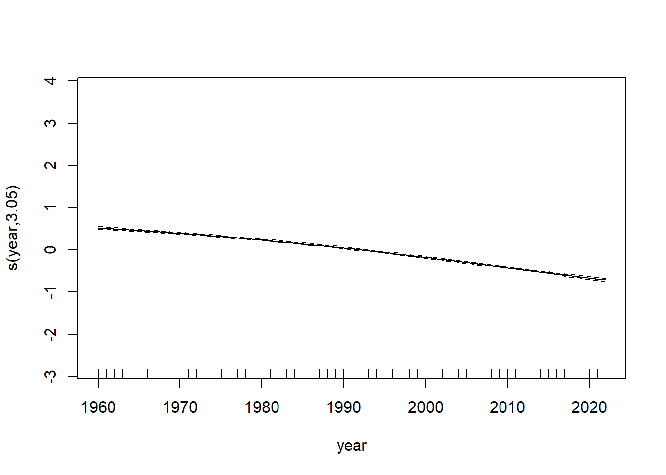

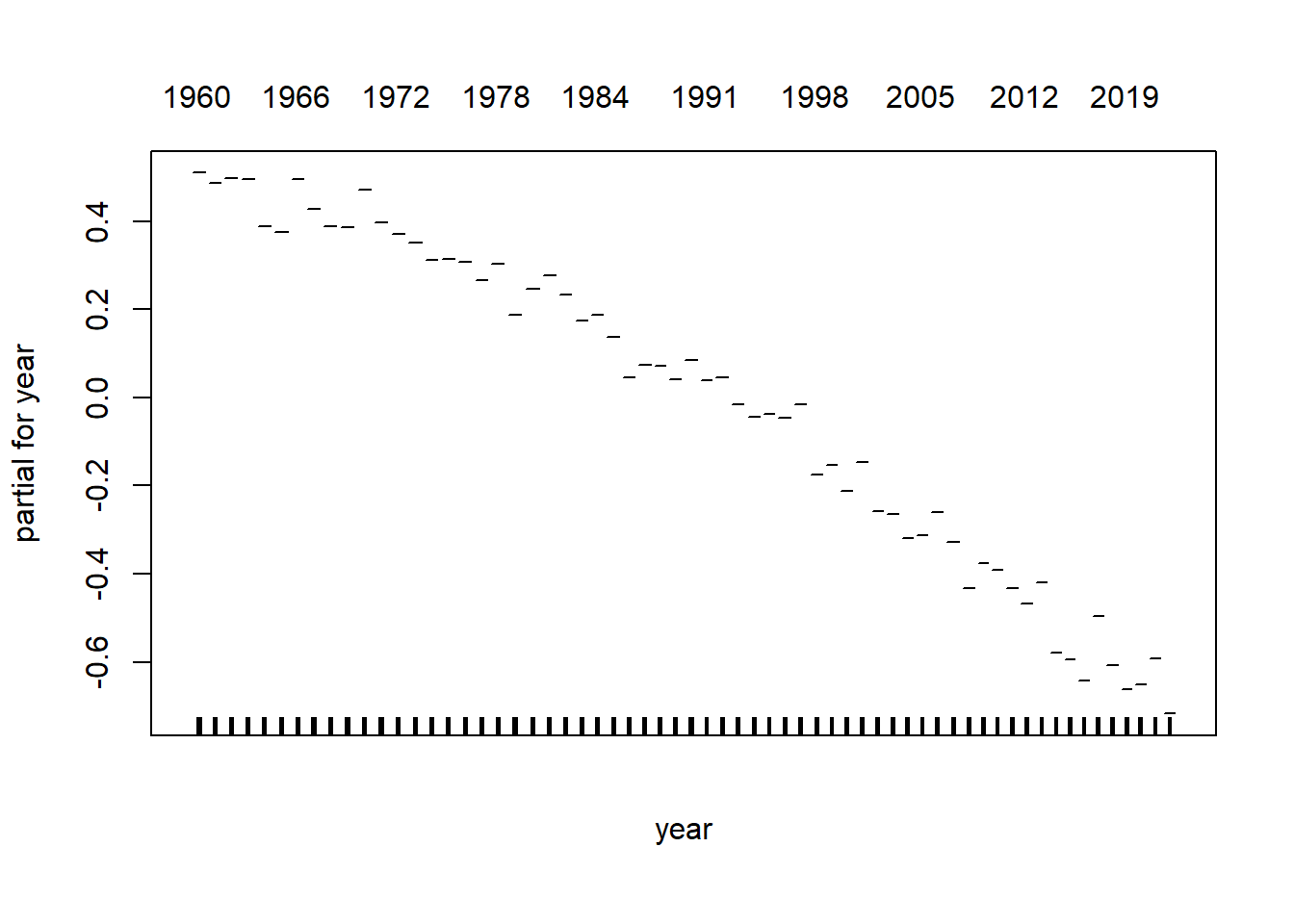
GAMs on Luxembourg data (using gam package)

library(gam)
lux_factor <- lux %>% mutate(year = factor(year))
model_gam <- gam(log_mx ~ s(age) + year, data=lux_factor)
plot(model_gam)

Source: xkcd

Glossary

• interpolation & extrapolation
• polynomial regression
  • monomials
  • orthogonal polynomials
• step functions
  • basis function expansion
  • piecewise polynomial functions

• regression splines
  • knots
  • natural splines
  • cubic splines
• smoothing splines
• local regression
• generalised additive models (GAMs)

Recommended viewing (splines)

The Continuity of Splines

It won’t help with your assessment, it’s just very entertaining/interesting.

Recommended viewing (LOESS)

What is LOESS and When Should I Use It?

R Package versions

print(sessionInfo(), locale=FALSE, tzone=FALSE)

R version 4.5.0 (2025-04-11 ucrt)
Platform: x86_64-w64-mingw32/x64
Running under: Windows 11 x64 (build 26100)

Matrix products: default
  LAPACK version 3.12.1

attached base packages:
[1] splines   stats     graphics  grDevices utils     datasets  methods  
[8] base     

other attached packages:
 [1] gam_1.22-5      foreach_1.5.2   glue_1.8.0      plotly_4.10.4  
 [5] mgcv_1.9-1      nlme_3.1-168    lubridate_1.9.4 forcats_1.0.0  
 [9] stringr_1.5.1   dplyr_1.1.4     purrr_1.0.4     readr_2.1.5    
[13] tidyr_1.3.1     tibble_3.2.1    ggplot2_3.5.2   tidyverse_2.0.0

loaded via a namespace (and not attached):
 [1] generics_0.1.4     stringi_1.8.7      lattice_0.22-6     hms_1.1.3         
 [5] digest_0.6.37      magrittr_2.0.3     evaluate_1.0.3     grid_4.5.0        
 [9] timechange_0.3.0   RColorBrewer_1.1-3 iterators_1.0.14   fastmap_1.2.0     
[13] rprojroot_2.0.4    jsonlite_2.0.0     Matrix_1.7-3       httr_1.4.7        
[17] crosstalk_1.2.1    viridisLite_0.4.2  scales_1.4.0       codetools_0.2-20  
[21] lazyeval_0.2.2     cli_3.6.5          rlang_1.1.6        withr_3.0.2       
[25] yaml_2.3.10        tools_4.5.0        tzdb_0.5.0         here_1.0.1        
[29] reticulate_1.42.0  vctrs_0.6.5        R6_2.6.1           png_0.1-8         
[33] lifecycle_1.0.4    htmlwidgets_1.6.4  pkgconfig_2.0.3    pillar_1.10.2     
[37] gtable_0.3.6       data.table_1.17.2  Rcpp_1.0.14        xfun_0.52         
[41] tidyselect_1.2.1   knitr_1.50         farver_2.1.2       htmltools_0.5.8.1 
[45] rmarkdown_2.29     labeling_0.4.3     compiler_4.5.0    

Python Package versions

from watermark import watermark
print(watermark(python=True, packages="matplotlib,numpy,pandas,seaborn,scipy"))

Python implementation: CPython
Python version       : 3.11.12
IPython version      : 9.2.0

matplotlib: 3.10.3
numpy     : 2.2.6
pandas    : 2.2.3
seaborn   : 0.13.2
scipy     : 1.15.3

References

James, G., Witten, D., Hastie, T., & Tibshirani, R. (2021). An Introduction to Statistical Learning: with Applications in R. Springer.