USArrests.hist <- hclust(dist(USArrests), method = "complete")
plot(USArrests.hist)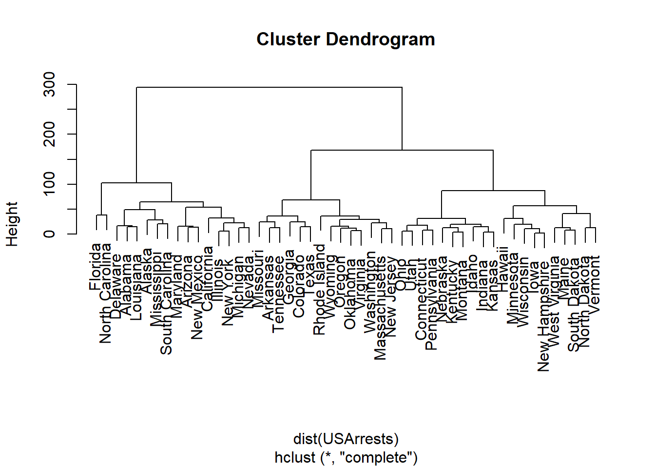
Questions about PCA were sourced from the excellent textbook Géron (2022), which is available through the UNSW Library’s access to O’Reilly Media texts. The author also provided a Google Colab notebook containing the coding solutions.
\star Solution (ISLR2, Q9.2) Suppose that we have four observations, for which we compute a dissimilarity matrix, given by \begin{aligned} \begin{bmatrix} & 0.3 & 0.4 & 0.7 \\ 0.3 & & 0.5 & 0.8 \\ 0.4 & 0.5 & & 0.45 \\ 0.7 & 0.8 & 0.45 & \end{bmatrix} \end{aligned} For instance, the dissimilarity between the first and second observations is 0.3, and the dissimilarity between the second and fourth observations is 0.8.
On the basis of this dissimilarity matrix, sketch the dendrogram that results from hierarchically clustering these four observations using complete linkage. Be sure to indicate on the plot the height at which each fusion occurs, as well as the observations corresponding to each leaf in the dendrogram.
Repeat (a), this time using single linkage clustering.
Suppose that we cut the dendrogram obtained in (a) such that two clusters result. Which observations are in each cluster?
Suppose that we cut the dendrogram obtained in (b) such that two clusters result. Which observations are in each cluster?
It is mentioned in the chapter that at each fusion in the dendrogram, the position of the two clusters being fused can be swapped without changing the meaning of the dendrogram. Draw a dendrogram that is equivalent to the dendrogram in (a), for which two or more of the leaves are repositioned, but for which the meaning of the dendrogram is the same.
\star Solution (ISLR2, Q9.3) In this problem, you will perform K-means clustering manually, with K = 2, on a small example with n = 6 observations and p = 2 features. The observations are as follows.
| Obs | X_1 | X_2 |
|---|---|---|
| 1 | 1 | 4 |
| 2 | 1 | 3 |
| 3 | 0 | 4 |
| 4 | 5 | 1 |
| 5 | 6 | 2 |
| 6 | 4 | 0 |
Plot the observations.
Randomly assign a cluster label to each observation. You can use the sample() command in R to do this. Report the cluster labels for each observation.
Compute the centroid for each cluster.
Assign each observation to the centroid to which it is closest, in terms of Euclidean distance. Report the cluster labels for each observation.
Repeat (c) and (d) until the answers obtained stop changing.
In your plot from (a), color the observations according to the cluster labels obtained.
\star Solution (HandsOnML3, Q8.1) What are the main motivations for reducing a dataset’s dimensionality? What are the main drawbacks?
\star Solution (HandsOnML3, Q8.3) Once a dataset’s dimensionality has been reduced, is it possible to reverse the operation? If so, how? If not, why?
Solution (HandsOnML3, Q8.4) Can PCA be used to reduce the dimensionality of a highly nonlinear dataset?
\star Solution (HandsOnML3, Q8.5) Suppose you perform PCA on a 1,000-dimensional dataset, setting the explained variance ratio to 95%. How many dimensions will the resulting dataset have?
Solution (HandsOnML3, Q8.7) How can you evaluate the performance of a dimensionality reduction algorithm on your dataset?
\star Solution (ISLR2, Q9.9) Consider the USArrests data. We will now perform hierarchical clustering on the states.
Using hierarchical clustering with complete linkage and Euclidean distance, cluster the states.
Cut the dendrogram at a height that results in three distinct clusters. Which states belong to which clusters?
Hierarchically cluster the states using complete linkage and Euclidean distance, after scaling the variables to have standard deviation one.
What effect does scaling the variables have on the hierarchical clustering obtained? In your opinion, should the variables be scaled before the inter-observation dissimilarities are computed? Provide a justification for your answer.
Solution (ISLR2, Q9.13) On the book website, www.statlearning.com, there is a gene expression data set (Ch12Ex13.csv) that consists of 40 tissue samples with measurements on 1,000 genes. The first 20 samples are from healthy patients, while the second 20 are from a diseased group.
Load in the data using read.csv(). You will need to select header = F.
Apply hierarchical clustering to the samples using correlationbased distance, and plot the dendrogram. Do the genes separate the samples into the two groups? Do your results depend on the type of linkage used?
Solution Load the MNIST data sets (uploaded as two CSV files) from the course website. Note we use a training set that is smaller than the entire data (only 10,000 of the 60,000 training instances). The test set is another 10,000 observations. Train a random forest classifier on the dataset and time how long it takes, then evaluate the resulting model on the test set. Next, use PCA to reduce the dataset’s dimensionality, with an explained variance ratio of 95%. Train a new random forest classifier on the reduced dataset and see how long it takes. Was training much faster? Next, evaluate the classifier on the test set. How does it compare to the previous classifier? Try again with a SGDClassifier (if using Python) or a kNN (if using R). How much does PCA help now?
See Figure 1

See Figure 2

(1,2), (3,4)
(1, 2, 3), (4)
See Figure 3

See Figure 4

See Table 1.
| Obs. | X_1 | X_2 | Label |
|---|---|---|---|
| 1 | 1 | 4 | 1 |
| 2 | 1 | 3 | 1 |
| 3 | 0 | 4 | 2 |
| 4 | 5 | 1 | 2 |
| 5 | 6 | 2 | 1 |
| 6 | 4 | 0 | 2 |
Label 1 X_1 = 2.67, X_2 = 3.00
Label 2 X_1 = 3.00, X_2 = 1.67
See Table 2.
| Obs. | X_1 | X_2 | Label |
|---|---|---|---|
| 1 | 1 | 4 | 1 |
| 2 | 1 | 3 | 1 |
| 3 | 0 | 4 | 1 |
| 4 | 5 | 1 | 2 |
| 5 | 6 | 2 | 2 |
| 6 | 4 | 0 | 2 |
See Figure 5

Question The main motivations for dimensionality reduction are:
The main drawbacks are:
Question Once a dataset’s dimensionality has been reduced using one of the algorithms we discussed, it is almost always impossible to perfectly reverse the operation, because some information gets lost during dimensionality reduction. Moreover, while some algorithms (such as PCA) have a simple reverse transformation procedure that can reconstruct a dataset relatively similar to the original, other algorithms (such as t-SNE) do not.
Question PCA can be used to significantly reduce the dimensionality of most datasets, even if they are highly nonlinear, because it can at least get rid of useless dimensions. However, if there are no useless dimensions—as in the Swiss roll dataset—then reducing dimensionality with PCA will lose too much information. You want to unroll the Swiss roll, not squash it.
Question That’s a trick question: it depends on the dataset. Let’s look at two extreme examples. First, suppose the dataset is composed of points that are almost perfectly aligned. In this case, PCA can reduce the dataset down to just one dimension while still preserving 95% of the variance. Now imagine that the dataset is composed of perfectly random points, scattered all around the 1,000 dimensions. In this case roughly 950 dimensions are required to preserve 95% of the variance. So the answer is, it depends on the dataset, and it could be any number between 1 and 950. Plotting the explained variance as a function of the number of dimensions is one way to get a rough idea of the dataset’s intrinsic dimensionality.
Question Intuitively, a dimensionality reduction algorithm performs well if it eliminates a lot of dimensions from the dataset without losing too much information. One way to measure this is to apply the reverse transformation and measure the reconstruction error. However, not all dimensionality reduction algorithms provide a reverse transformation. Alternatively, if you are using dimensionality reduction as a preprocessing step before another Machine Learning algorithm (e.g., a Random Forest classifier), then you can simply measure the performance of that second algorithm; if dimensionality reduction did not lose too much information, then the algorithm should perform just as well as when using the original dataset.
USArrests.hist <- hclust(dist(USArrests), method = "complete")
plot(USArrests.hist)
cutree(USArrests.hist, 3) Alabama Alaska Arizona Arkansas California
1 1 1 2 1
Colorado Connecticut Delaware Florida Georgia
2 3 1 1 2
Hawaii Idaho Illinois Indiana Iowa
3 3 1 3 3
Kansas Kentucky Louisiana Maine Maryland
3 3 1 3 1
Massachusetts Michigan Minnesota Mississippi Missouri
2 1 3 1 2
Montana Nebraska Nevada New Hampshire New Jersey
3 3 1 3 2
New Mexico New York North Carolina North Dakota Ohio
1 1 1 3 3
Oklahoma Oregon Pennsylvania Rhode Island South Carolina
2 2 3 2 1
South Dakota Tennessee Texas Utah Vermont
3 2 2 3 3
Virginia Washington West Virginia Wisconsin Wyoming
2 2 3 3 2 USArrests.scale <- scale(USArrests, center = FALSE, scale = TRUE)
USArrests.scale.hist <- hclust(dist(USArrests.scale))
plot(USArrests.scale.hist)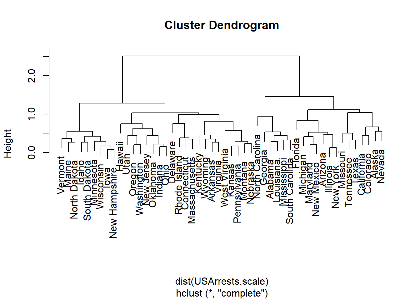
murder much rarer than assault), it seems especially relevant to scale.# Note that you will have to download the csv file into your working
# directory
myData <- read.csv("Ch12Ex13.csv", header = FALSE)gene.cluster <- hclust(as.dist(1 - cor(myData)), method = "complete")
plot(gene.cluster)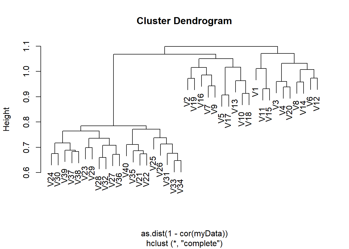
library(randomForest)
library(rbenchmark)
library(caret)
library(kknn)
Exercise: Load the MNIST dataset
mnist_train <- read.csv("mnist_small_train.csv")
X_train <- mnist_train[, -1]
y_train <- as.factor(mnist_train[, "label"])

mnist_test <- read.csv("mnist_test.csv")
X_test <- mnist_test[, -1]
y_test <- as.factor(mnist_test[, "label"])

# Some of the columns have zero variance, so we remove them
nonzero_var_cols <- which(apply(X_train, 2, var) != 0)
X_train <- X_train[, nonzero_var_cols]
X_test <- X_test[, nonzero_var_cols]
Exercise: Train a Random Forest classifier on the dataset and time how long it takes, then evaluate the resulting model on the test set.
benchmark(
  rnd_clf <- randomForest(X_train, y_train,
                          ntree=20, seed=42, maxnodes=100),
  replications=1)
y_pred <- predict(rnd_clf, X_test)
accuracy_score <- sum(y_pred == y_test) / length(y_test)
accuracy_score[1] 0.8868Exercise: Next, use PCA to reduce the dataset’s dimensionality, with an explained variance ratio of 95%.
pca <- preProcess(X_train, method=c("pca"), thresh=0.95)
X_train_reduced <- predict(pca, X_train)
X_test_reduced <- predict(pca, X_test)
ncol(X_train_reduced)
[1] 284Exercise: Train a new Random Forest classifier on the reduced dataset and see how long it takes. Was training much faster?
benchmark(
  rnd_clf_with_pca <- randomForest(X_train_reduced, y_train,
                                           ntree=20, seed=42, maxnodes=100),
  replications=1
)
Training time is better: “elapsed” time reduced by a factor of more than 2, which is a notable improvement. That said, please note that dimensionality reduction does not always lead to faster training time: it depends on the dataset, the model and the training algorithm. See Figure 8-6 in Géron (2022). We next check the precision of the new random forest classifier.
Exercise: Next evaluate the classifier on the test set: how does it compare to the previous classifier (that uses the “original” data)?
y_pred <- predict(rnd_clf_with_pca, X_test_reduced)
accuracy_score <- sum(y_pred == y_test) / length(y_test)
accuracy_score
[1] 0.7992It is common for performance to drop slightly when reducing dimensionality, because we do lose some potentially useful signal in the process. However, the performance drop is rather severe in this case. So PCA results are mixed: while the fitting was faster, it yielded reduced performance.
Exercise: Try again with an KNNClassifier. How much does PCA help now?
# The train.kknn function takes a formula as input
df_train <- data.frame(y = y_train, X_train)[1:5000,]

# Fit the model
benchmark(
  knn_model <- train.kknn(y ~ ., data = df_train, ks=1:4),
  replications=1
)
# You can then predict with this model using the test data like so:
df_test <- data.frame(X_test)
predictions <- predict(knn_model, newdata = df_test)Warning in model.matrix.default(mt2, test, contrasts.arg = contrasts.arg):
variable 'y' is absent, its contrast will be ignoredaccuracy_score <- sum(predictions == y_test) / length(y_test)
accuracy_score[1] 0.8952Okay, so the KNNClassifier takes much longer to train on this dataset than the RandomForestClassifier (and its predictive performance on the test set is similar to the Random Forest model). But that’s not what we are interested in right now, we want to see how much PCA can help KNNClassifier.
Exercise: Let’s train it using the reduced dataset:
df_train <- data.frame(y = y_train, X_train_reduced)[1:5000,]

benchmark(
  knn_model <- train.kknn(y ~ ., data = df_train, ks=1:4),
  replications=1
)
df_test <- data.frame(X_test_reduced)
predictions <- predict(knn_model, newdata = df_test)Warning in model.matrix.default(mt2, test, contrasts.arg = contrasts.arg):
variable 'y' is absent, its contrast will be ignoredaccuracy_score <- sum(predictions == y_test) / length(y_test)
accuracy_score[1] 0.7935Again, we have a speed boost (elapsed time reduced), at the cost of a substantial reduction in performance.
Exercise: Load the MNIST dataset
import pandas as pd

mnist_train = pd.read_csv("mnist_small_train.csv")
X_train = mnist_train.drop("label", axis=1)
y_train = mnist_train["label"]

mnist_test = pd.read_csv("mnist_test.csv")
X_test = mnist_test.drop("label", axis=1)
y_test = mnist_test["label"]
Exercise: Train a Random Forest classifier on the dataset and time how long it takes, then evaluate the resulting model on the test set.
from sklearn.ensemble import RandomForestClassifier
from timeit import default_timer as timer

rnd_clf = RandomForestClassifier(n_estimators=100, random_state=42)

start = timer()
rnd_clf.fit(X_train, y_train);
print(timer() - start)3.7110771000006935from sklearn.metrics import accuracy_score
y_pred = rnd_clf.predict(X_test)
accuracy_score(y_test, y_pred)0.9514Exercise: Next, use PCA to reduce the dataset’s dimensionality, with an explained variance ratio of 95%.
from sklearn.decomposition import PCA

pca = PCA(n_components=0.95)
X_train_reduced = pca.fit_transform(X_train)
Exercise: Train a new Random Forest classifier on the reduced dataset and see how long it takes. Was training much faster?
rnd_clf_with_pca = RandomForestClassifier(n_estimators=100, random_state=42)

start = timer()
rnd_clf_with_pca.fit(X_train_reduced, y_train);
print(timer() - start)15.492053599999963Oh no! Training is actually about twice slower now! How can that be? Well, as we saw in this chapter, dimensionality reduction does not always lead to faster training time: it depends on the dataset, the model and the training algorithm. See Figure 8-6. If you try SGDClassifier instead of RandomForestClassifier, you will find that training time is reduced by a factor of 5 when using PCA. Actually, we will do this in a second, but first let’s check the precision of the new random forest classifier.
Exercise: Next evaluate the classifier on the test set: how does it compare to the previous classifier?
X_test_reduced = pca.transform(X_test)

y_pred = rnd_clf_with_pca.predict(X_test_reduced)
accuracy_score(y_test, y_pred)0.9131It is common for performance to drop slightly when reducing dimensionality, because we do lose some potentially useful signal in the process. However, the performance drop is rather severe in this case. So PCA really did not help: it slowed down training and reduced performance. 😭
It is common for performance to drop slightly when reducing dimensionality, because we do lose some potentially useful signal in the process. However, the performance drop is rather severe in this case. So PCA really did not help: it slowed down training and reduced performance. :’(
Exercise: Try again with an SGDClassifier. How much does PCA help now?
from sklearn.linear_model import SGDClassifier

sgd_clf = SGDClassifier(random_state=42)

start = timer()
sgd_clf.fit(X_train, y_train);
print(timer() - start)4.7651230999999825y_pred = sgd_clf.predict(X_test)
accuracy_score(y_test, y_pred)0.8919Okay, so the SGDClassifier takes much longer to train on this dataset than the RandomForestClassifier, plus it performs worse on the test set. But that’s not what we are interested in right now, we want to see how much PCA can help SGDClassifier. Let’s train it using the reduced dataset:
sgd_clf_with_pca = SGDClassifier(random_state=42)
start = timer()
sgd_clf_with_pca.fit(X_train_reduced, y_train);
print(timer() - start)1.0539340999994238Nice! Reducing dimensionality led to roughly 5× speedup. :) Let’s check the model’s accuracy:
y_pred = sgd_clf_with_pca.predict(X_test_reduced)
accuracy_score(y_test, y_pred)0.8965Great! PCA not only gave us a roughly 5x speed boost, it also improved performance slightly.
So there you have it: PCA can give you a formidable speedup, and if you’re lucky a performance boost… but it’s really not guaranteed: it depends on the model and the dataset!