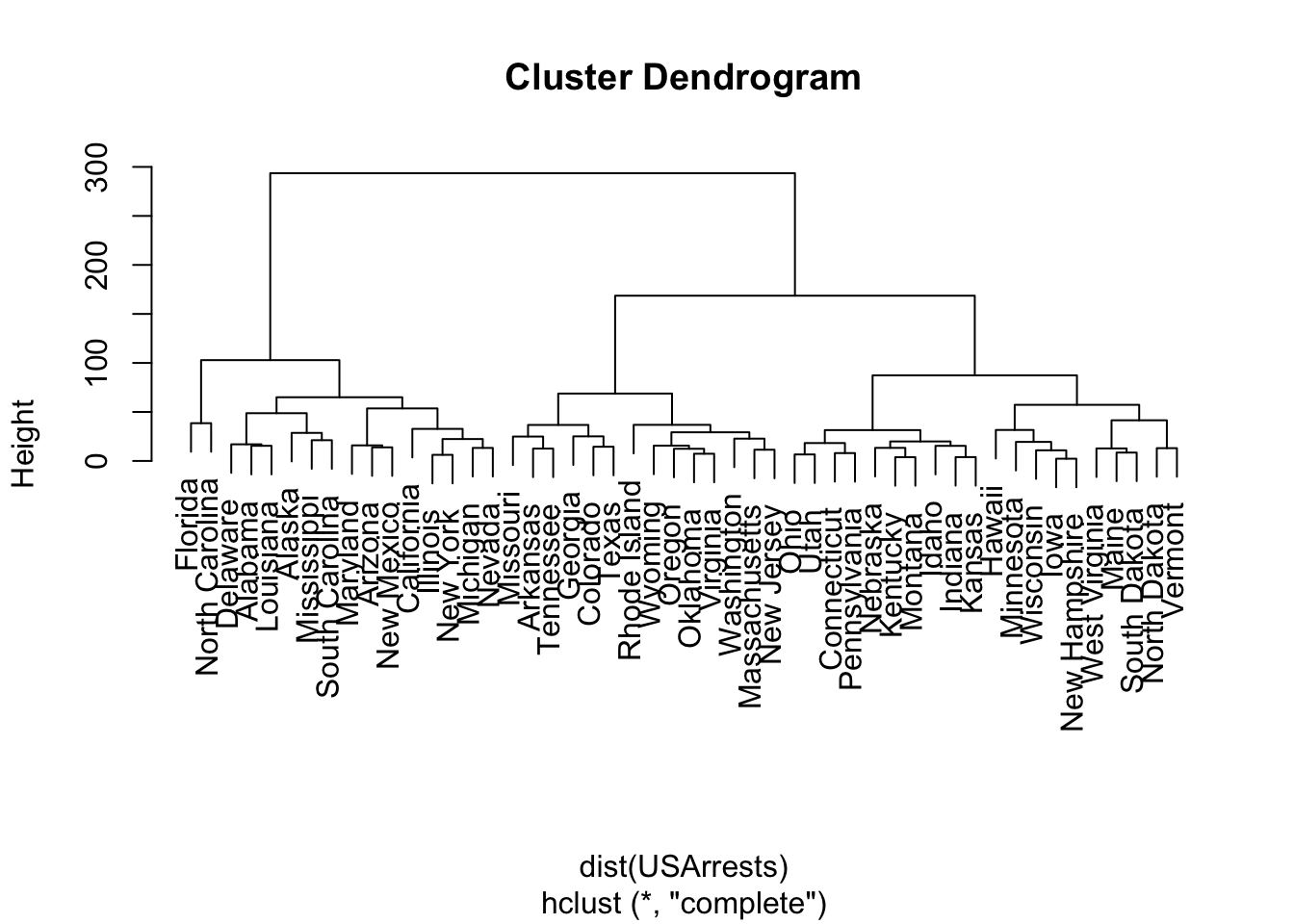
USArrests.hist <- hclust(dist(USArrests), method = "complete")
plot(USArrests.hist)
(ISLR2, Q9.2) Suppose that we have four observations, for which we compute a dissimilarity matrix, given by For instance, the dissimilarity between the first and second observations is 0.3, and the dissimilarity between the second and fourth observations is 0.8.
On the basis of this dissimilarity matrix, sketch the dendrogram that results from hierarchically clustering these four observations using complete linkage. Be sure to indicate on the plot the height at which each fusion occurs, as well as the observations corresponding to each leaf in the dendrogram.
Repeat (a), this time using single linkage clustering.
Suppose that we cut the dendrogram obtained in (a) such that two clusters result. Which observations are in each cluster?
Suppose that we cut the dendrogram obtained in (b) such that two clusters result. Which observations are in each cluster?
It is mentioned in the chapter that at each fusion in the dendrogram, the position of the two clusters being fused can be swapped without changing the meaning of the dendrogram. Draw a dendrogram that is equivalent to the dendrogram in (a), for which two or more of the leaves are repositioned, but for which the meaning of the dendrogram is the same.
(ISLR2, Q9.3) In this problem, you will perform -means clustering manually, with , on a small example with observations and features. The observations are as follows.
| Obs | ||
|---|---|---|
| 1 | 1 | 4 |
| 2 | 1 | 3 |
| 3 | 0 | 4 |
| 4 | 5 | 1 |
| 5 | 6 | 2 |
| 6 | 4 | 0 |
Plot the observations.
Randomly assign a cluster label to each observation. You can use the sample() command in R to do this. Report the cluster labels for each observation.
Compute the centroid for each cluster.
Assign each observation to the centroid to which it is closest, in terms of Euclidean distance. Report the cluster labels for each observation.
Repeat (c) and (d) until the answers obtained stop changing.
In your plot from (a), color the observations according to the cluster labels obtained.
In hierarchical clustering, two dissimilarity measures have been mentioned: Euclidean and correlation.
Consider two vectors and
Their Euclidean dissimilarity is:
For the correlation dissimilarity, we treat values as if they are from the same distribution and values as if they are from the same distribution . Hence, there correlation dissimilarity is
Show that, in the case where and , correlation dissimilarity and Euclidean dissimilarity give the same results. (Use the population variance instead of the sample variance)
Provide a geometric interpretation of the correlation dissimilarity and the Euclidean dissimilarity. When would each be appropriate?
(ISLR2, Q9.9) Consider the USArrests data. We will now perform hierarchical clustering on the states.
Using hierarchical clustering with complete linkage and Euclidean distance, cluster the states.
Cut the dendrogram at a height that results in three distinct clusters. Which states belong to which clusters?
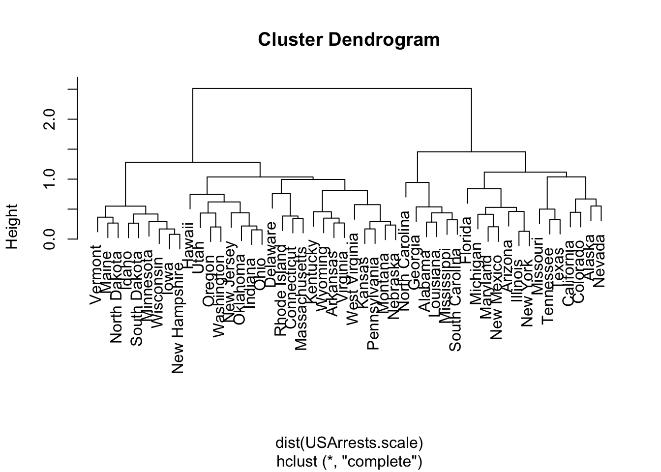
Hierarchically cluster the states using complete linkage and Euclidean distance, after scaling the variables to have standard deviation one.
What effect does scaling the variables have on the hierarchical clustering obtained? In your opinion, should the variables be scaled before the inter-observation dissimilarities are computed? Provide a justification for your answer.
(ISLR2, Q9.13) On the book website, www.statlearning.com, there is a gene expression data set (Ch12Ex13.csv) that consists of 40 tissue samples with measurements on 1,000 genes. The first 20 samples are from healthy patients, while the second 20 are from a diseased group.
Load in the data using read.csv(). You will need to select header = F.
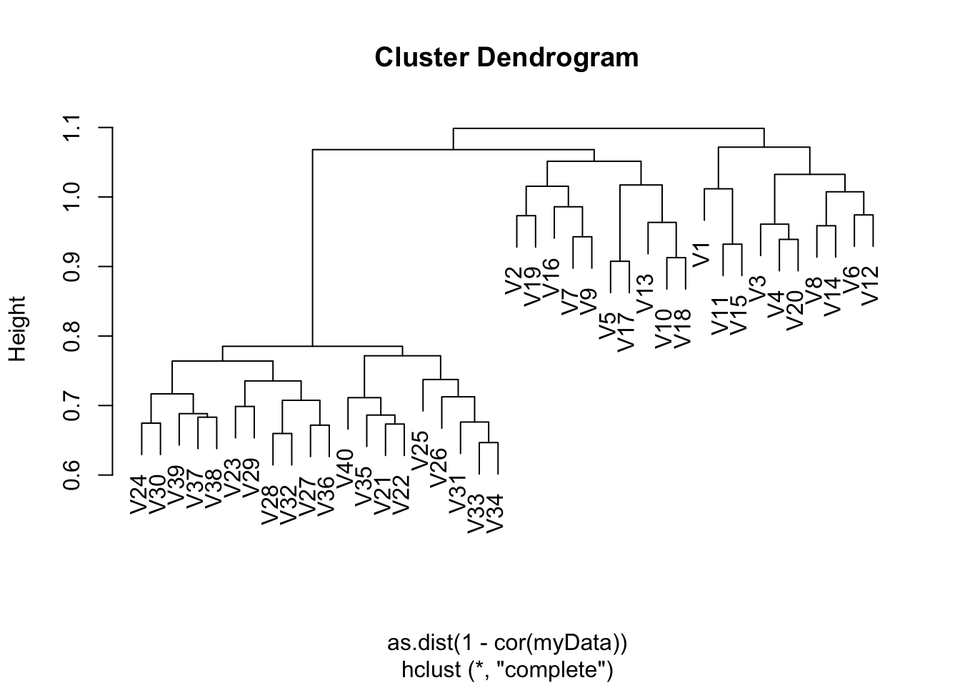
Apply hierarchical clustering to the samples using correlationbased distance, and plot the dendrogram. Do the genes separate the samples into the two groups? Do your results depend on the type of linkage used?
Breaking down the Euclidean dissimilarity: Noting that .
Now breaking down the Correlation dissimilarity: This is directly proportional to the Euclidean dissimilarity, and thus will give the same results (provided the method is linear in the way it summarises).
Euclidean dissimilarity looks at how close the points are to each other in the parameter space, so if the data is clustered and related data tends to be of the same order of magnitude, this is appropriate. Correlation dissimilarity looks at how well the points fit on the same line. This is more appropriate if similar changes in features indicate similarity, despite the values being rather different.
USArrests.hist <- hclust(dist(USArrests), method = "complete")
plot(USArrests.hist)
cutree(USArrests.hist, 3) Alabama Alaska Arizona Arkansas California
1 1 1 2 1
Colorado Connecticut Delaware Florida Georgia
2 3 1 1 2
Hawaii Idaho Illinois Indiana Iowa
3 3 1 3 3
Kansas Kentucky Louisiana Maine Maryland
3 3 1 3 1
Massachusetts Michigan Minnesota Mississippi Missouri
2 1 3 1 2
Montana Nebraska Nevada New Hampshire New Jersey
3 3 1 3 2
New Mexico New York North Carolina North Dakota Ohio
1 1 1 3 3
Oklahoma Oregon Pennsylvania Rhode Island South Carolina
2 2 3 2 1
South Dakota Tennessee Texas Utah Vermont
3 2 2 3 3
Virginia Washington West Virginia Wisconsin Wyoming
2 2 3 3 2 USArrests.scale <- scale(USArrests, center = FALSE, scale = TRUE)
USArrests.scale.hist <- hclust(dist(USArrests.scale))
plot(USArrests.scale.hist)
# Note that you will have to download the csv file into your working
# directory
myData <- read.csv("Ch12Ex13.csv", header = FALSE)
gene.cluster <- hclust(as.dist(1 - cor(myData)), method = "complete")
plot(gene.cluster)